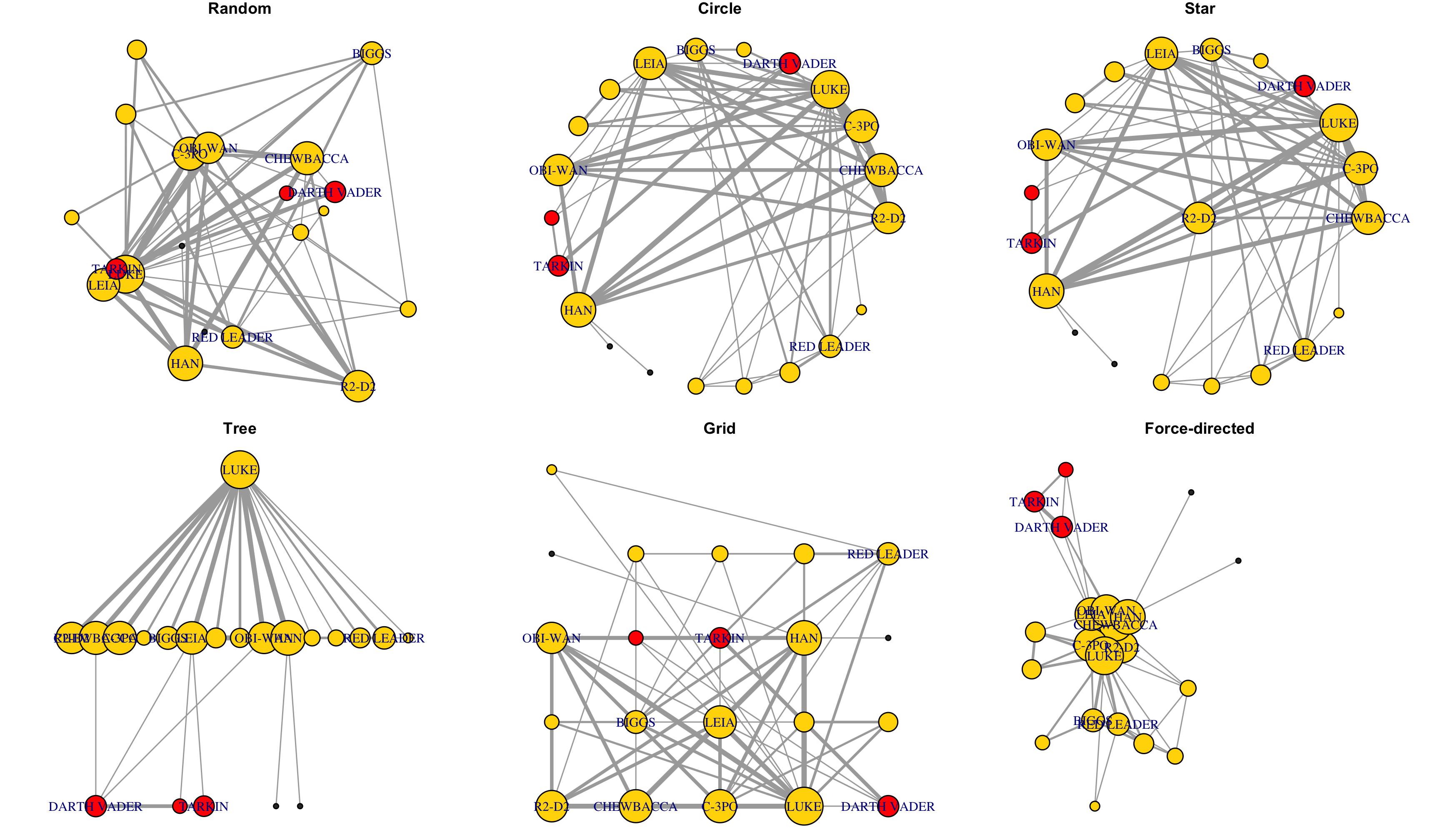
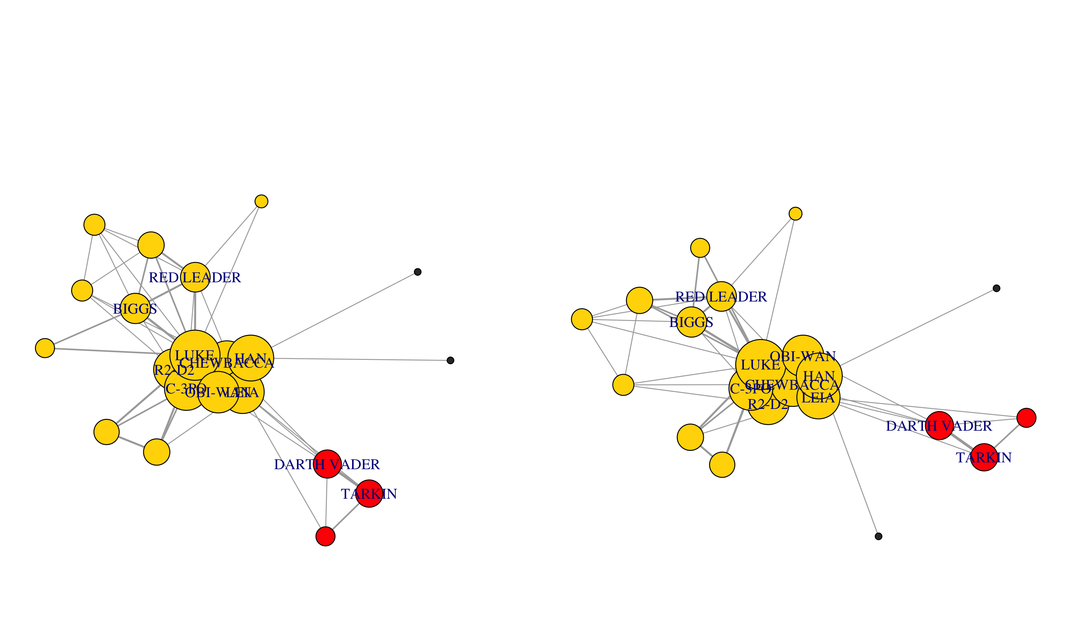
The Social Network
A Note
This will be a crash course so if you don’t get everything, that is fine! Hopefully this sparks some interest in the idea of network analysis.
Node and Network Properties
What are the most important nodes in a network? What is the propensity of two nodes that are connected to be both connected to a third node? What are the different hidden communities in a network? These are some of the descriptive questions that we will address.
We’ll start with descriptive statistics at the node level. All of these are in some way measures of importance or centrality.
The most basic measure is degree, the number of adjacent edges to each node. It is often considered a measure of direct influence. In the Star Wars network, it will be the unique number of characters that each character is interacting with.
sort(degree(g))## GOLD FIVE GREEDO JABBA CAMIE RED TEN OWEN
## 0 1 1 2 2 3
## MOTTI TARKIN BERU DARTH VADER DODONNA GOLD LEADER
## 3 3 4 5 5 5
## WEDGE R2-D2 BIGGS OBI-WAN RED LEADER CHEWBACCA
## 5 7 7 7 7 8
## HAN C-3PO LEIA LUKE
## 8 10 12 15In directed graphs, there are three types of degree: indegree (incoming edges), outdegree (outgoing edges), and total degree. You can find these using mode="in" or mode="out" or mode="total".
Strength is a weighted measure of degree that takes into account the number of edges that go from one node to another. In this network, it will be the total number of interactions of each character with anybody else.
sort(strength(g))## GOLD FIVE GREEDO JABBA RED TEN CAMIE MOTTI
## 0 1 1 2 4 4
## DODONNA GOLD LEADER OWEN BERU WEDGE TARKIN
## 5 5 8 9 9 10
## DARTH VADER RED LEADER BIGGS OBI-WAN R2-D2 LEIA
## 11 13 14 49 50 59
## CHEWBACCA C-3PO HAN LUKE
## 63 64 80 129Closeness measures how many steps are required to access every other node from a given node. It’s a measure of how long information takes to arrive (who hears news first?). Higher values mean less centrality.
sort(closeness(g, normalized=TRUE))## Warning in closeness(g, normalized = TRUE): At centrality.c:2617 :closeness
## centrality is not well-defined for disconnected graphs## GOLD FIVE GREEDO JABBA HAN OWEN CAMIE
## 0.04545455 0.11666667 0.11666667 0.13043478 0.17647059 0.18584071
## TARKIN R2-D2 OBI-WAN MOTTI DARTH VADER BERU
## 0.20000000 0.20388350 0.20792079 0.21000000 0.21649485 0.21649485
## CHEWBACCA WEDGE RED TEN C-3PO LUKE LEIA
## 0.21875000 0.21875000 0.22105263 0.23595506 0.23863636 0.24418605
## GOLD LEADER RED LEADER DODONNA BIGGS
## 0.24418605 0.25000000 0.25301205 0.25925926Betweenness measures brokerage or gatekeeping potential. It is (approximately) the number of shortest paths between nodes that pass through a particular node.
sort(betweenness(g))## CAMIE OWEN OBI-WAN MOTTI TARKIN GREEDO
## 0.000000 0.000000 0.000000 0.000000 0.000000 0.000000
## JABBA WEDGE GOLD FIVE BERU RED TEN DARTH VADER
## 0.000000 0.000000 0.000000 1.666667 2.200000 15.583333
## CHEWBACCA LUKE R2-D2 GOLD LEADER RED LEADER BIGGS
## 15.916667 18.333333 22.750000 23.800000 31.416667 31.916667
## C-3PO HAN DODONNA LEIA
## 32.783333 37.000000 47.533333 59.950000Eigenvector centrality is a measure of being well-connected connected to the well-connected. I’ll spare you the linear algebra lesson but this only works with undirected networks.
sort(eigen_centrality(g)$vector)## MOTTI TARKIN JABBA GREEDO RED TEN GOLD LEADER
## 0.009298153 0.011493184 0.011602602 0.011602604 0.015241796 0.017475057
## DARTH VADER CAMIE DODONNA WEDGE OWEN RED LEADER
## 0.027009389 0.030744983 0.031723524 0.034374377 0.062695673 0.065141246
## BERU BIGGS GOLD FIVE R2-D2 OBI-WAN LEIA
## 0.070824006 0.078921422 0.121485774 0.503053912 0.541729368 0.592624857
## C-3PO CHEWBACCA HAN LUKE
## 0.595864470 0.657663375 0.812242325 1.000000000Page rank approximates probability that any message will arrive to a particular node. This algorithm was developed by Google founders, and originally applied to website links.
sort(page_rank(g)$vector)## GOLD FIVE JABBA GREEDO RED TEN CAMIE DODONNA
## 0.007092199 0.008310156 0.008310156 0.010573836 0.013792262 0.016185680
## MOTTI GOLD LEADER OWEN BERU WEDGE TARKIN
## 0.016813964 0.017945853 0.018881975 0.020368818 0.026377242 0.034180007
## DARTH VADER RED LEADER BIGGS OBI-WAN R2-D2 LEIA
## 0.034576040 0.034578060 0.035070288 0.067378471 0.068538690 0.086027500
## CHEWBACCA C-3PO HAN LUKE
## 0.086390090 0.088708430 0.114631333 0.185268949Authority score is another measure of centrality initially applied to the Web. A node has high authority when it is linked by many other nodes that are linking many other nodes.
sort(authority_score(g)$vector)## GOLD FIVE MOTTI TARKIN GREEDO JABBA RED TEN
## 1.273708e-17 9.118469e-03 1.133319e-02 1.154515e-02 1.154515e-02 1.512880e-02
## GOLD LEADER DARTH VADER CAMIE DODONNA WEDGE OWEN
## 1.717615e-02 2.671707e-02 3.064953e-02 3.143121e-02 3.410098e-02 6.256707e-02
## RED LEADER BERU BIGGS R2-D2 OBI-WAN LEIA
## 6.476889e-02 7.063977e-02 7.856101e-02 5.030995e-01 5.417666e-01 5.923767e-01
## C-3PO CHEWBACCA HAN LUKE
## 5.957835e-01 6.577603e-01 8.125507e-01 1.000000e+00Finally, not exactly a measure of centrality, but we can learn more about who each node is connected to by using the following functions: neighbors (for direct neighbors) and ego (for neighbors up to n neighbors away)
neighbors(g, v=which(V(g)$name=="DARTH VADER"))## + 5/22 vertices, named, from ac319ee:
## [1] CHEWBACCA LEIA OBI-WAN MOTTI TARKINego(g, order=2, nodes=which(V(g)$name=="DARTH VADER"))## [[1]]
## + 14/22 vertices, named, from ac319ee:
## [1] DARTH VADER CHEWBACCA LEIA OBI-WAN MOTTI TARKIN
## [7] R2-D2 C-3PO LUKE HAN DODONNA BIGGS
## [13] BERU RED LEADERLet’s now try to describe what a network looks like as a whole. We can start with measures of the size of a network. diameter is the length of the longest path (in number of edges) between two nodes. We can use get_diameter to identify this path. mean_distance is the average number of edges between any two nodes in the network. We can find each of these paths between pairs of edges with distances.
diameter(g, directed=FALSE, weights=NA)## [1] 3get_diameter(g, directed=FALSE, weights=NA)## + 4/22 vertices, named, from ac319ee:
## [1] DARTH VADER CHEWBACCA C-3PO OWENmean_distance(g, directed=FALSE)## [1] 1.909524dist <- distances(g, weights=NA)
dist[1:5, 1:5]## R2-D2 CHEWBACCA C-3PO LUKE DARTH VADER
## R2-D2 0 1 1 1 2
## CHEWBACCA 1 0 1 1 1
## C-3PO 1 1 0 1 2
## LUKE 1 1 1 0 2
## DARTH VADER 2 1 2 2 0edge_density is the proportion of edges in the network over all possible edges that could exist.
edge_density(g)## [1] 0.2597403# 22*21 possible edges / 2 because it's undirected = 231 possible edges
# but only 60 exist
60/((22*21)/2)## [1] 0.2597403reciprocity measures the propensity of each edge to be a mutual edge; that is, the probability that if i is connected to j, j is also connected to i.
reciprocity(g)## [1] 1# Why is it 1?transitivity, also known as clustering coefficient, measures that probability that adjacent nodes of a network are connected. In other words, if i is connected to j, and j is connected to k, what is the probability that i is also connected to k?
transitivity(g)## [1] 0.5375303Network communities
Networks often have different clusters or communities of nodes that are more densely connected to each other than to the rest of the network. Let’s cover some of the different existing methods to identify these communities.
The most straightforward way to partition a network is into connected components. Each component is a group of nodes that are connected to each other, but not to the rest of the nodes. For example, this network has two components.
components(g)## $membership
## R2-D2 CHEWBACCA C-3PO LUKE DARTH VADER CAMIE
## 1 1 1 1 1 1
## BIGGS LEIA BERU OWEN OBI-WAN MOTTI
## 1 1 1 1 1 1
## TARKIN HAN GREEDO JABBA DODONNA GOLD LEADER
## 1 1 1 1 1 1
## WEDGE RED LEADER RED TEN GOLD FIVE
## 1 1 1 2
##
## $csize
## [1] 21 1
##
## $no
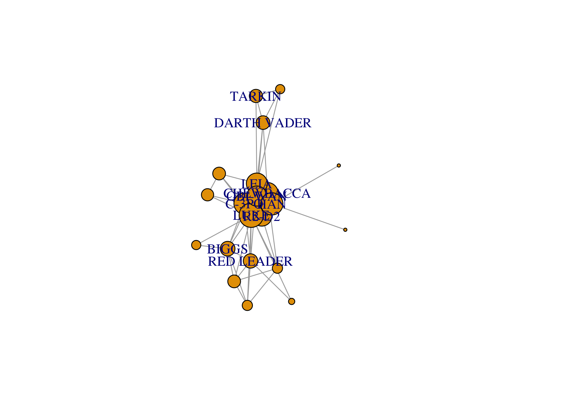
## [1] 2par(mar=c(0,0,0,0)); plot(g)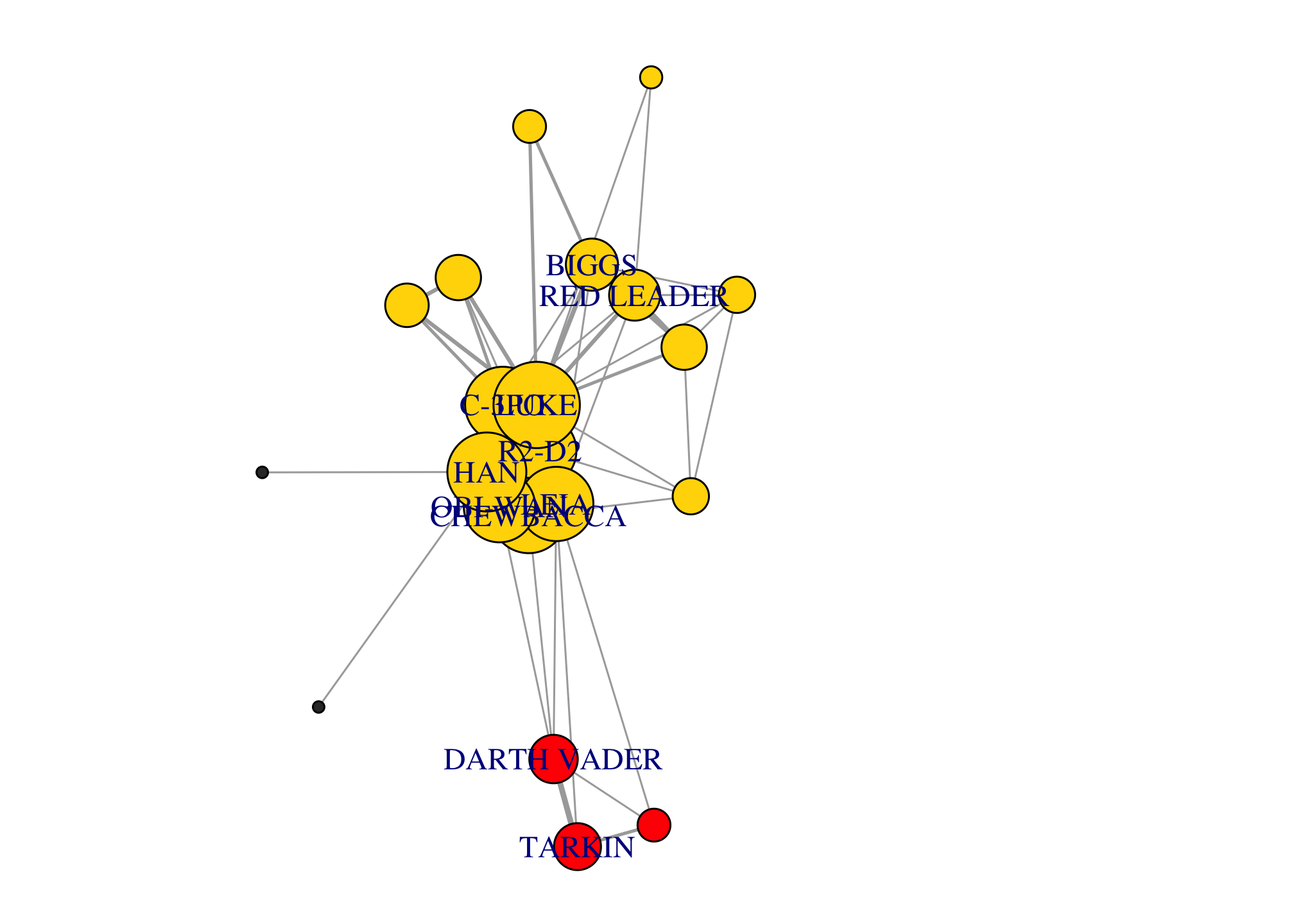
Most networks have a single giant connected component that includes most nodes. Most studies of networks actually focus on the giant component (e.g. the shortest path between nodes in a network with two or more component is Inf!).
giant <- decompose(g)[[1]]Components can be weakly connected (in undirected networks) or __strongly connected (in directed networks, where there is an edge that ends in every single node of that component).
Even within a giant component, there can be different subsets of the network that are more connected to each other than to the rest of the network. The goal of community detection algorithms is to identify these subsets.
There are a few different algorithms, each following a different logic.
The walktrap algorithm finds communities through a series of short random walks. The idea is that these random walks tend to stay within the same community. The length of these random walks is 4 edges by default, but you may want to experiment with different values. The goal of this algorithm is to identify the partition that maximizes a modularity score.
cluster_walktrap(giant)## IGRAPH clustering walktrap, groups: 6, mod: 0.16
## + groups:
## $`1`
## [1] "CAMIE" "BIGGS" "DODONNA" "GOLD LEADER" "WEDGE"
## [6] "RED LEADER" "RED TEN"
##
## $`2`
## [1] "DARTH VADER" "MOTTI" "TARKIN"
##
## $`3`
## [1] "R2-D2" "CHEWBACCA" "C-3PO" "LUKE" "LEIA" "OBI-WAN"
## [7] "HAN"
## + ... omitted several groups/verticescluster_walktrap(giant, steps=10)## IGRAPH clustering walktrap, groups: 3, mod: 0.15
## + groups:
## $`1`
## [1] "DARTH VADER" "MOTTI" "TARKIN"
##
## $`2`
## [1] "R2-D2" "CHEWBACCA" "C-3PO" "LUKE" "LEIA" "BERU"
## [7] "OWEN" "OBI-WAN" "HAN" "GREEDO" "JABBA"
##
## $`3`
## [1] "CAMIE" "BIGGS" "DODONNA" "GOLD LEADER" "WEDGE"
## [6] "RED LEADER" "RED TEN"
## + ... omitted several groups/verticesOther methods are:
- The fast and greedy method tries to directly optimize this modularity score.
- The infomap method attempts to map the flow of information in a network, and the different clusters in which information may get remain for longer periods. Similar to walktrap, but not necessarily maximizing modularity, but rather the so-called “map equation”.
- The edge-betweenness method iteratively removes edges with high betweenness, with the idea that they are likely to connect different parts of the network. Here betweenness (gatekeeping potential) applies to edges, but the intuition is the same.
- The label propagation method labels each node with unique labels, and then updates these labels by choosing the label assigned to the majority of their neighbors, and repeat this iteratively until each node has the most common labels among its neighbors.
cluster_fast_greedy(giant)## IGRAPH clustering fast greedy, groups: 4, mod: 0.17
## + groups:
## $`1`
## [1] "CHEWBACCA" "LUKE" "LEIA" "OBI-WAN" "HAN" "GREEDO"
## [7] "JABBA"
##
## $`2`
## [1] "R2-D2" "C-3PO" "BERU" "OWEN"
##
## $`3`
## [1] "CAMIE" "BIGGS" "DODONNA" "GOLD LEADER" "WEDGE"
## [6] "RED LEADER" "RED TEN"
## + ... omitted several groups/verticescluster_edge_betweenness(giant)## Warning in cluster_edge_betweenness(giant): At community.c:460 :Membership
## vector will be selected based on the lowest modularity score.## Warning in cluster_edge_betweenness(giant): At community.c:467 :Modularity
## calculation with weighted edge betweenness community detection might not make
## sense -- modularity treats edge weights as similarities while edge betwenness
## treats them as distances## IGRAPH clustering edge betweenness, groups: 2, mod: 0.033
## + groups:
## $`1`
## [1] "R2-D2" "CHEWBACCA" "DARTH VADER" "LEIA" "OBI-WAN"
## [6] "MOTTI" "TARKIN" "HAN" "GREEDO" "JABBA"
##
## $`2`
## [1] "C-3PO" "LUKE" "CAMIE" "BIGGS" "BERU"
## [6] "OWEN" "DODONNA" "GOLD LEADER" "WEDGE" "RED LEADER"
## [11] "RED TEN"
## cluster_infomap(giant)## IGRAPH clustering infomap, groups: 2, mod: 0.064
## + groups:
## $`1`
## [1] "R2-D2" "CHEWBACCA" "C-3PO" "LUKE" "CAMIE"
## [6] "BIGGS" "LEIA" "BERU" "OWEN" "OBI-WAN"
## [11] "HAN" "GREEDO" "JABBA" "DODONNA" "GOLD LEADER"
## [16] "WEDGE" "RED LEADER" "RED TEN"
##
## $`2`
## [1] "DARTH VADER" "MOTTI" "TARKIN"
## cluster_label_prop(giant)## IGRAPH clustering label propagation, groups: 2, mod: 0.064
## + groups:
## $`1`
## [1] "R2-D2" "CHEWBACCA" "C-3PO" "LUKE" "CAMIE"
## [6] "BIGGS" "LEIA" "BERU" "OWEN" "OBI-WAN"
## [11] "HAN" "GREEDO" "JABBA" "DODONNA" "GOLD LEADER"
## [16] "WEDGE" "RED LEADER" "RED TEN"
##
## $`2`
## [1] "DARTH VADER" "MOTTI" "TARKIN"
## My experience is that infomap tends to work better in most social science examples (websites, social media, classrooms, etc), but fastgreedy is faster.
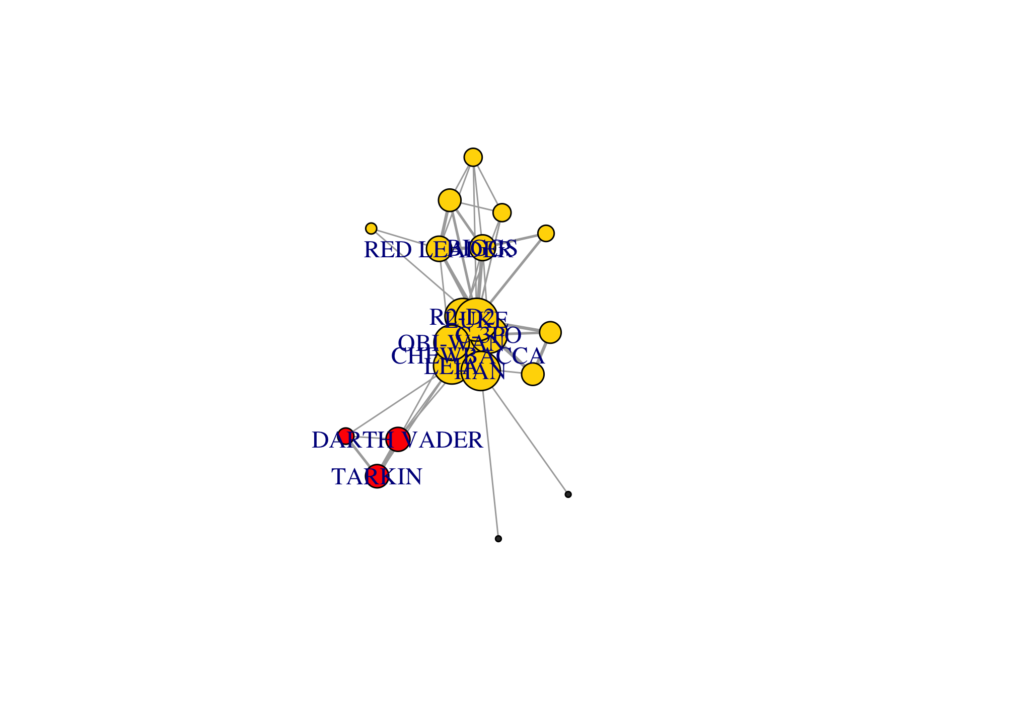
igraph also makes it very easy to plot the resulting communities:
comm <- cluster_infomap(giant)
modularity(comm) # modularity score
## [1] 0.06420569par(mar=c(0,0,0,0)); plot(comm, giant)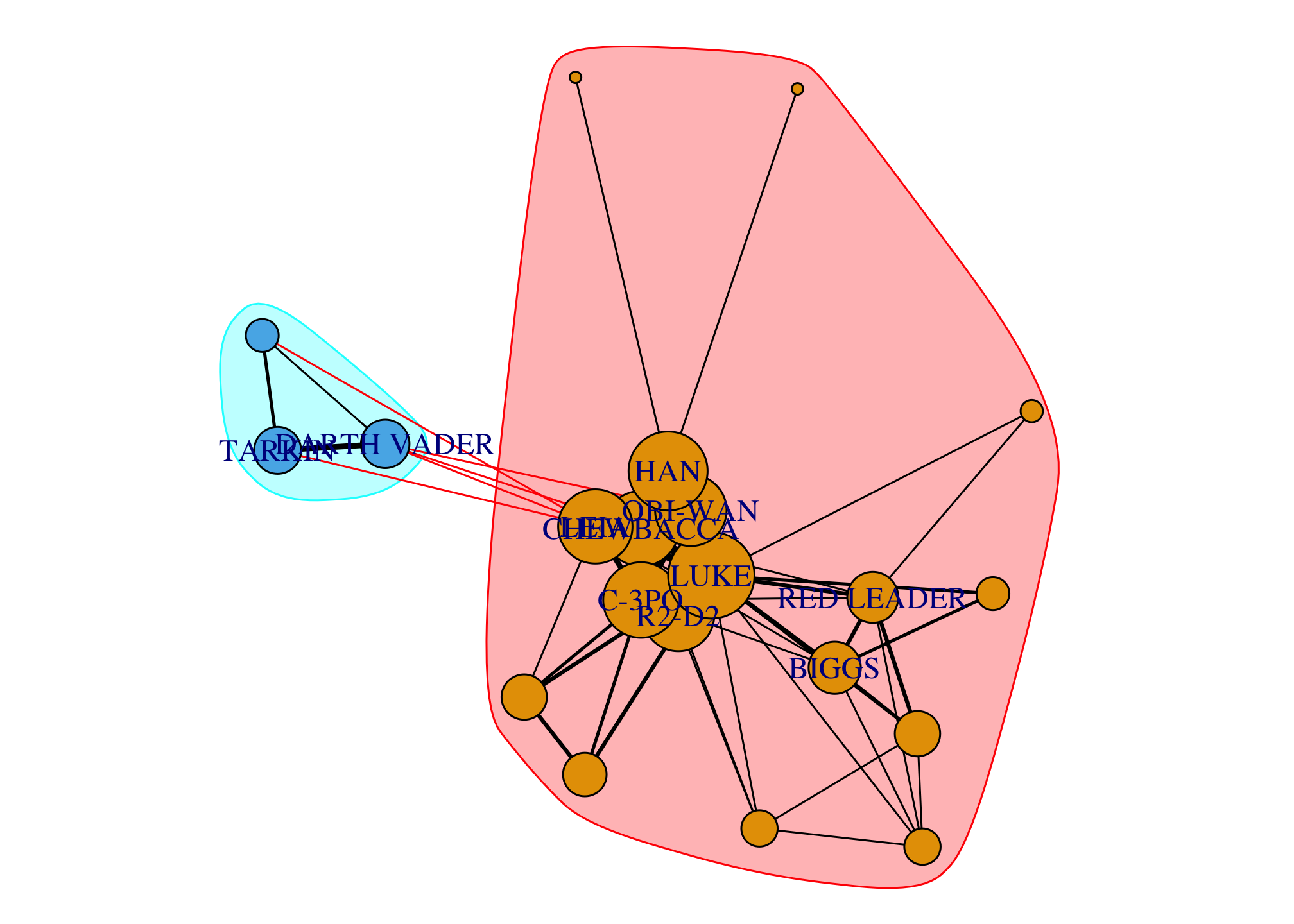
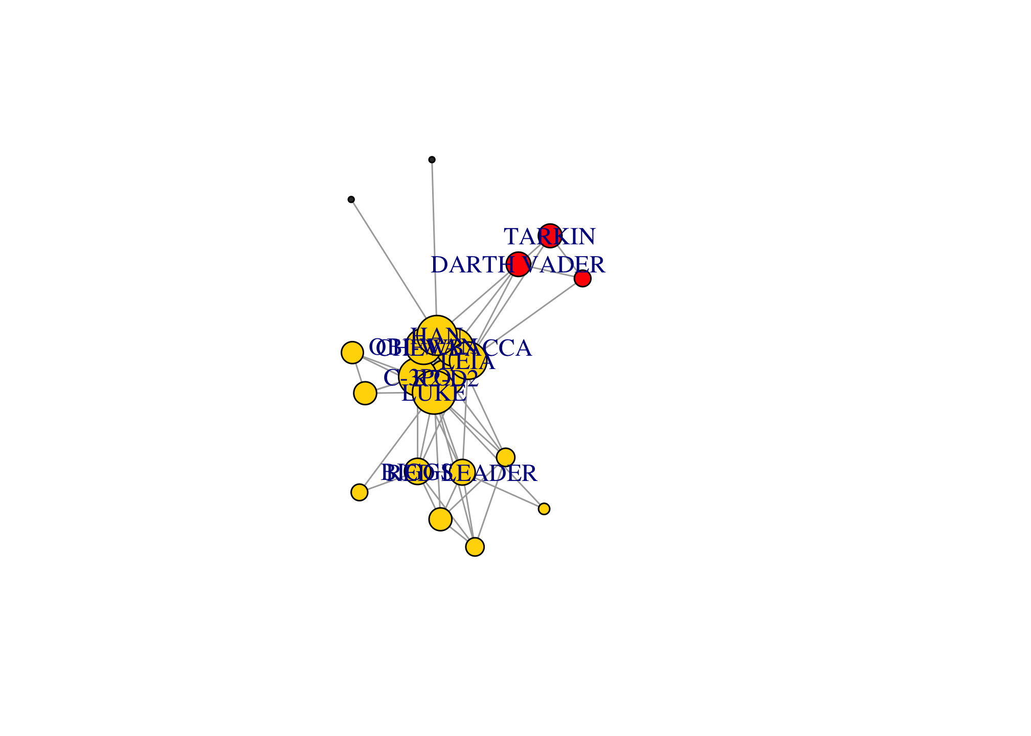
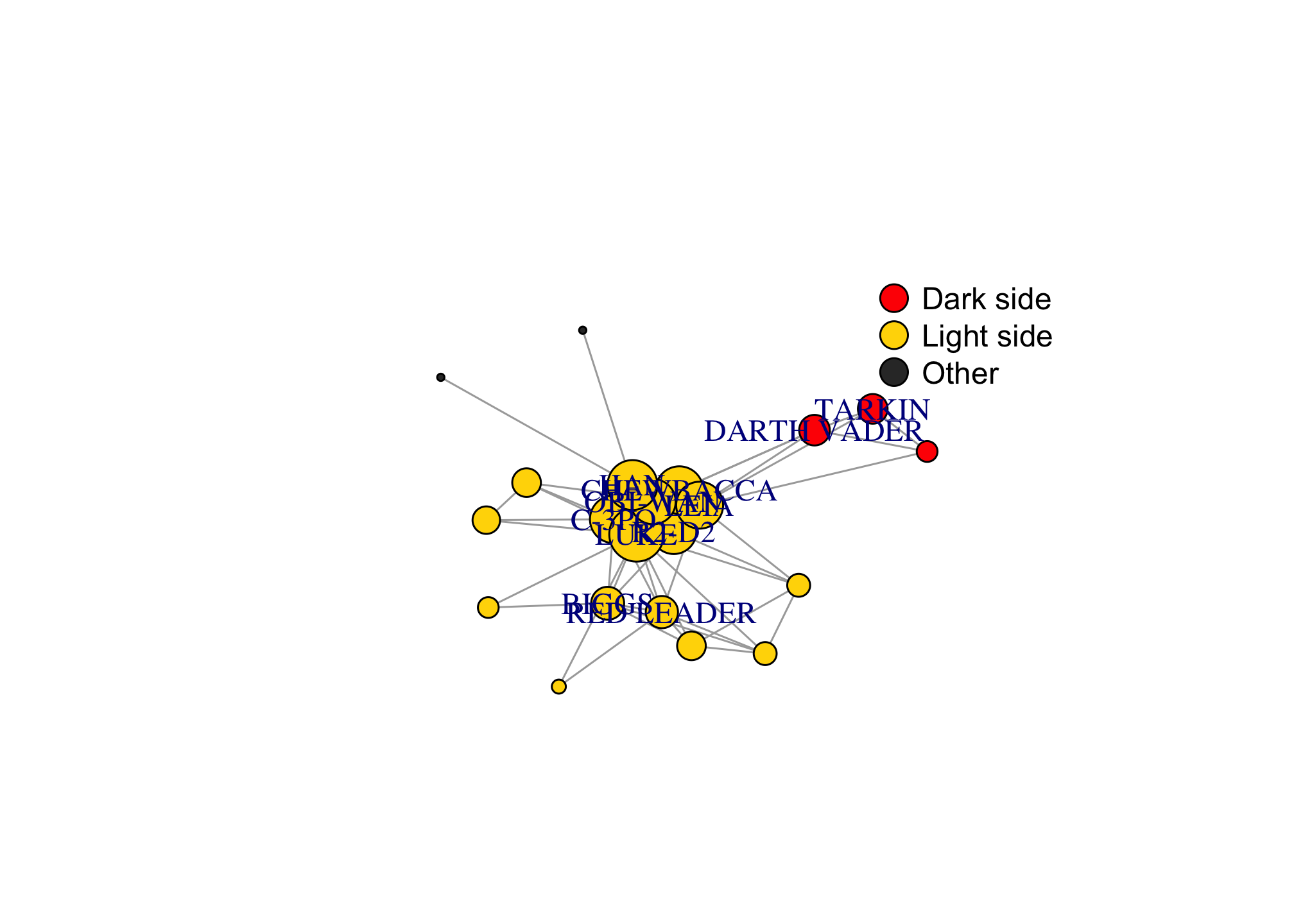
Alternatively, we can also add the membership to different communities as a color parameter in the igraph object.
V(giant)$color <- membership(comm)
par(mar=c(0,0,0,0)); plot(giant)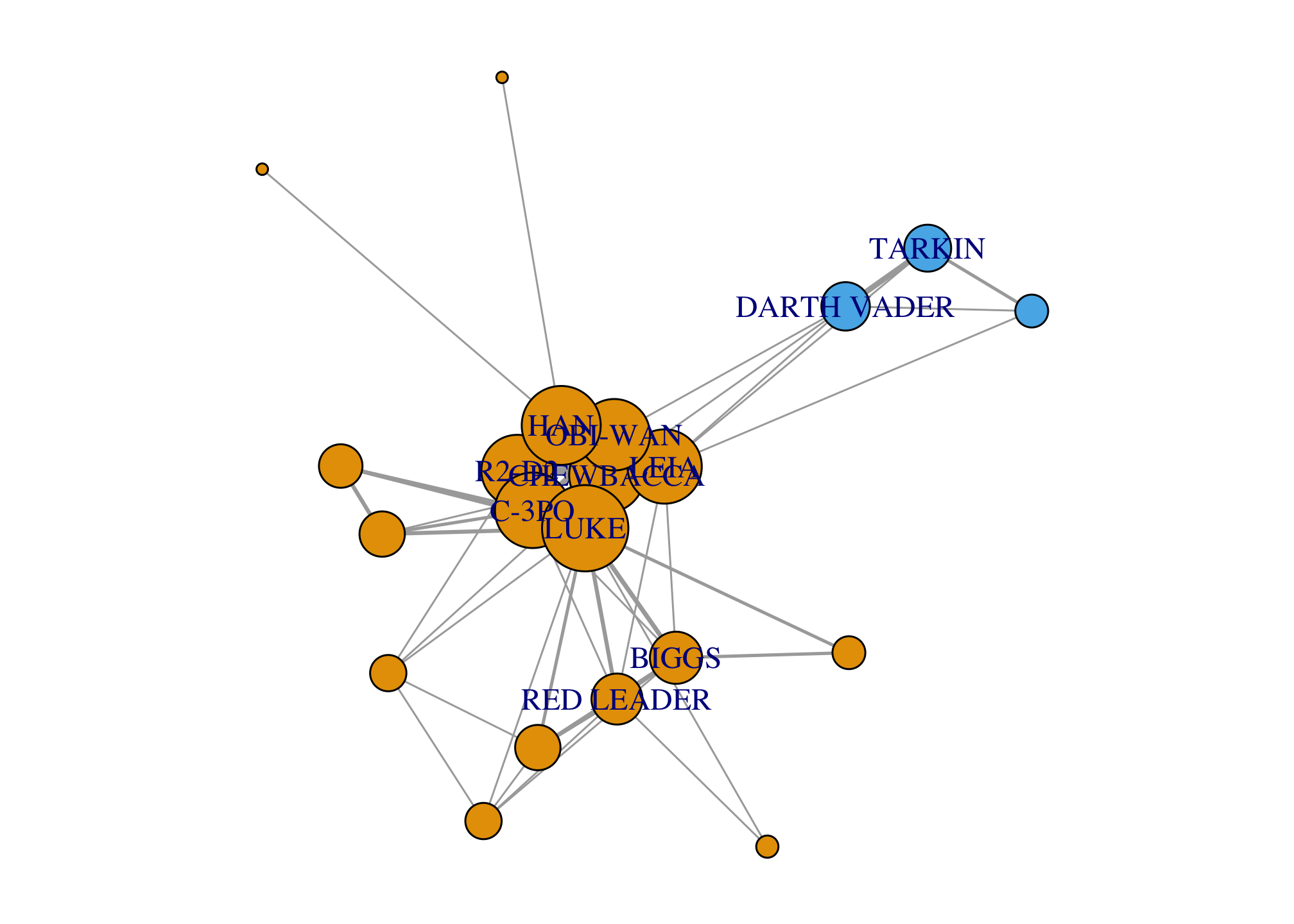
The final way in which we can think about network communities is in terms of hierarchy or structure. We’ll discuss two of these methods.
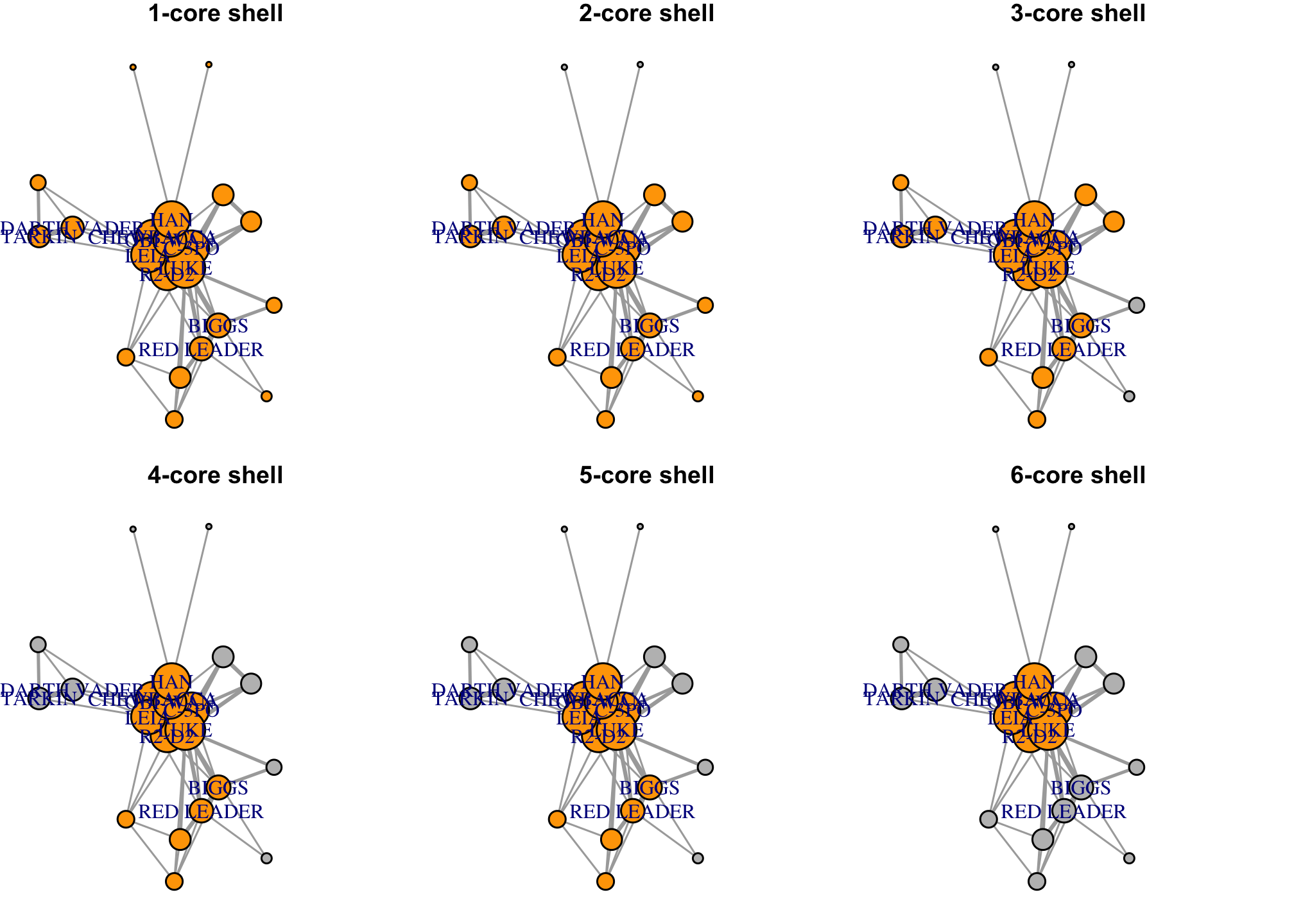
K-core decomposition allows us to identify the core and the periphery of the network. A k-core is a subnetwork where each node has degree k. So a 3-core would imply that each node is at least degree 3.
coreness(g)## R2-D2 CHEWBACCA C-3PO LUKE DARTH VADER CAMIE
## 6 6 6 6 3 2
## BIGGS LEIA BERU OWEN OBI-WAN MOTTI
## 5 6 3 3 6 3
## TARKIN HAN GREEDO JABBA DODONNA GOLD LEADER
## 3 6 1 1 5 5
## WEDGE RED LEADER RED TEN GOLD FIVE
## 5 5 2 0which(coreness(g)==6) # what is the core of the network?## R2-D2 CHEWBACCA C-3PO LUKE LEIA OBI-WAN HAN
## 1 2 3 4 8 11 14which(coreness(g)==1) # what is the periphery of the network?## GREEDO JABBA
## 15 16# Visualizing network structure
V(g)$coreness <- coreness(g)
par(mfrow=c(2, 3), mar=c(0.1,0.1,1,0.1))
set.seed(777); fr <- layout_with_fr(g)
for (k in 1:6){
V(g)$color <- ifelse(V(g)$coreness>=k, "orange", "grey")
plot(g, main=paste0(k, '-core shell'), layout=fr)
}
Getting tidy
library(tidyverse)Let’s remind ourselves of what the data looks like!
nodes## # A tibble: 22 x 3
## name id allegiance
## <chr> <dbl> <chr>
## 1 R2-D2 0 Galactic Republic
## 2 CHEWBACCA 1 Galactic Republic
## 3 C-3PO 2 Galactic Republic
## 4 LUKE 3 Jedi Order
## 5 DARTH VADER 4 Sith Order
## 6 CAMIE 5 Unknown
## 7 BIGGS 6 Galactic Republic
## 8 LEIA 7 Galactic Republic
## 9 BERU 8 Galactic Republic
## 10 OWEN 9 Galactic Republic
## # … with 12 more rowsedges## # A tibble: 60 x 3
## source target weight
## <chr> <chr> <dbl>
## 1 C-3PO R2-D2 17
## 2 LUKE R2-D2 13
## 3 OBI-WAN R2-D2 6
## 4 LEIA R2-D2 5
## 5 HAN R2-D2 5
## 6 CHEWBACCA R2-D2 3
## 7 DODONNA R2-D2 1
## 8 CHEWBACCA OBI-WAN 7
## 9 C-3PO CHEWBACCA 5
## 10 CHEWBACCA LUKE 16
## # … with 50 more rowsThe network package
Please install and load the following package
library(network)## network: Classes for Relational Data
## Version 1.16.1 created on 2020-10-06.
## copyright (c) 2005, Carter T. Butts, University of California-Irvine
## Mark S. Handcock, University of California -- Los Angeles
## David R. Hunter, Penn State University
## Martina Morris, University of Washington
## Skye Bender-deMoll, University of Washington
## For citation information, type citation("network").
## Type help("network-package") to get started.##
## Attaching package: 'network'## The following objects are masked from 'package:igraph':
##
## %c%, %s%, add.edges, add.vertices, delete.edges, delete.vertices,
## get.edge.attribute, get.edges, get.vertex.attribute, is.bipartite,
## is.directed, list.edge.attributes, list.vertex.attributes,
## set.edge.attribute, set.vertex.attributeThe command structure is not reall straight forward, but you can always enter ?network() into the console if you get confused.
As noted in the documentation, The first argument is a matrix giving the network structure in adjacency, incidence, or edgelist form.
The language demonstrates the significance of matrices in network analysis, but instead of a matrix, we have an edge list, which fills the same role. The second argument is a list of vertex attributes, which corresponds to the nodes list. Notice that similar to igraph,the network package uses the term vertices instead of nodes.
We then need to specify the type of data that has been entered into the first two arguments by specifying that the matrix.type is an edgelist Finally, we set ignore.eval to FALSE so that our network can be weighted and take into account the number of letters along each route.
starwars_network <-
  network(edges,
          vertex.attr = nodes,
          matrix.type = "edgelist",
          ignore.eval = FALSE)
and you can verify what it is by
class(starwars_network)## [1] "network"Printing out starwars_network to the console shows that the structure of the object is pretty different from data-frame style objects such as edges and nodes.
The print command reveals information that is specifically defined for network analysis. It shows that there are 21 vertices or nodes and 60 edges which we saw earlier. Again, these numbers correspond to the number of rows in nodes and edges respectively. Additionally like before, we can also see that the vertices and edges both contain attributes such as label and weight. You can get even more information, including what is known as a sociomatrix of the data, by entering
summary(starwars_network)## Network attributes:
## vertices = 21
## directed = TRUE
## hyper = FALSE
## loops = FALSE
## multiple = FALSE
## bipartite = FALSE
## total edges = 60
## missing edges = 0
## non-missing edges = 60
## density = 0.1428571
##
## Vertex attributes:
##
## allegiance:
## character valued attribute
## attribute summary:
## Galactic Empire Galactic Republic Hutt Cartel Jedi Order
## 2 13 2 2
## Sith Order Unknown
## 1 1
##
## id:
## numeric valued attribute
## attribute summary:
## Min. 1st Qu. Median Mean 3rd Qu. Max.
## 0 5 10 10 15 20
##
## name:
## character valued attribute
## attribute summary:
## the 10 most common values are:
## BERU BIGGS C-3PO CAMIE CHEWBACCA DARTH VADER
## 1 1 1 1 1 1
## DODONNA GOLD LEADER GREEDO HAN
## 1 1 1 1
## vertex.names:
## character valued attribute
## 21 valid vertex names
##
## Edge attributes:
##
## weight:
## numeric valued attribute
## attribute summary:
## Min. 1st Qu. Median Mean 3rd Qu. Max.
## 1.000 1.000 2.000 4.917 6.000 26.000
##
## Network edgelist matrix:
## [,1] [,2]
## [1,] 3 17
## [2,] 13 17
## [3,] 15 17
## [4,] 12 17
## [5,] 10 17
## [6,] 5 17
## [7,] 7 17
## [8,] 5 15
## [9,] 3 5
## [10,] 5 13
## [11,] 5 10
## [12,] 5 12
## [13,] 5 6
## [14,] 5 7
## [15,] 4 13
## [16,] 2 4
## [17,] 2 13
## [18,] 6 12
## [19,] 1 13
## [20,] 1 16
## [21,] 1 3
## [22,] 13 16
## [23,] 3 13
## [24,] 3 16
## [25,] 3 12
## [26,] 12 13
## [27,] 1 12
## [28,] 13 15
## [29,] 3 15
## [30,] 12 15
## [31,] 14 20
## [32,] 6 14
## [33,] 6 20
## [34,] 10 15
## [35,] 10 13
## [36,] 9 10
## [37,] 10 11
## [38,] 3 10
## [39,] 12 14
## [40,] 12 20
## [41,] 10 12
## [42,] 6 15
## [43,] 7 8
## [44,] 7 21
## [45,] 7 13
## [46,] 8 21
## [47,] 8 13
## [48,] 13 21
## [49,] 2 12
## [50,] 12 18
## [51,] 13 18
## [52,] 2 18
## [53,] 2 3
## [54,] 3 18
## [55,] 18 21
## [56,] 8 18
## [57,] 2 21
## [58,] 18 19
## [59,] 2 8
## [60,] 13 19which we can then visualize
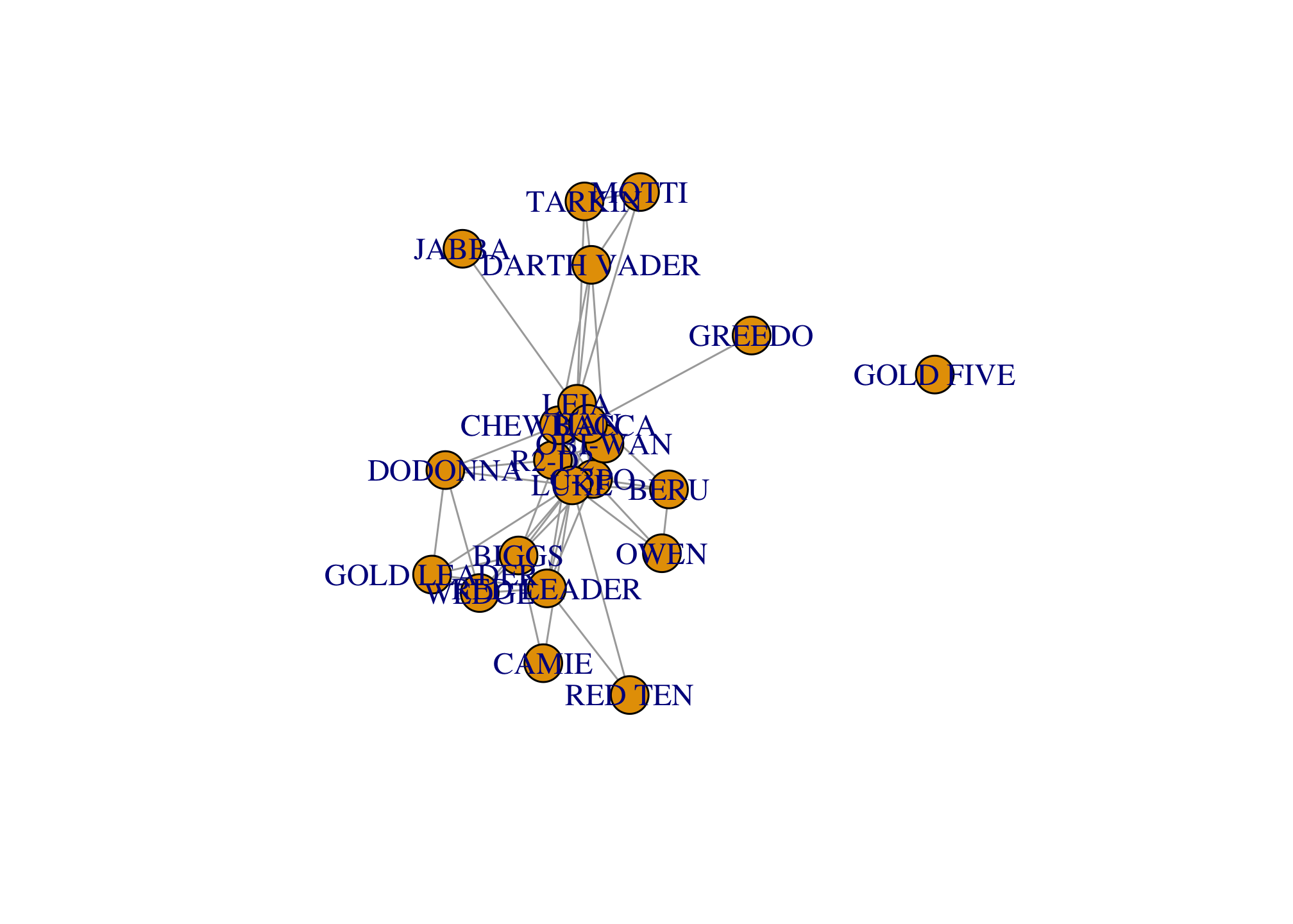
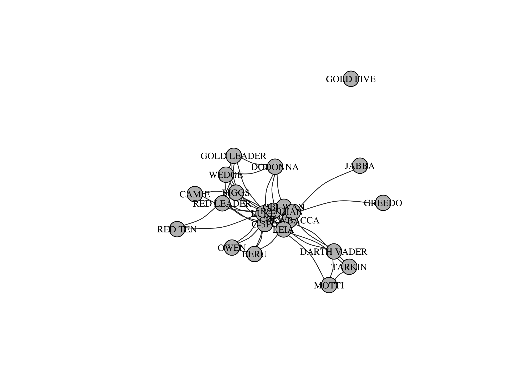
plot(starwars_network)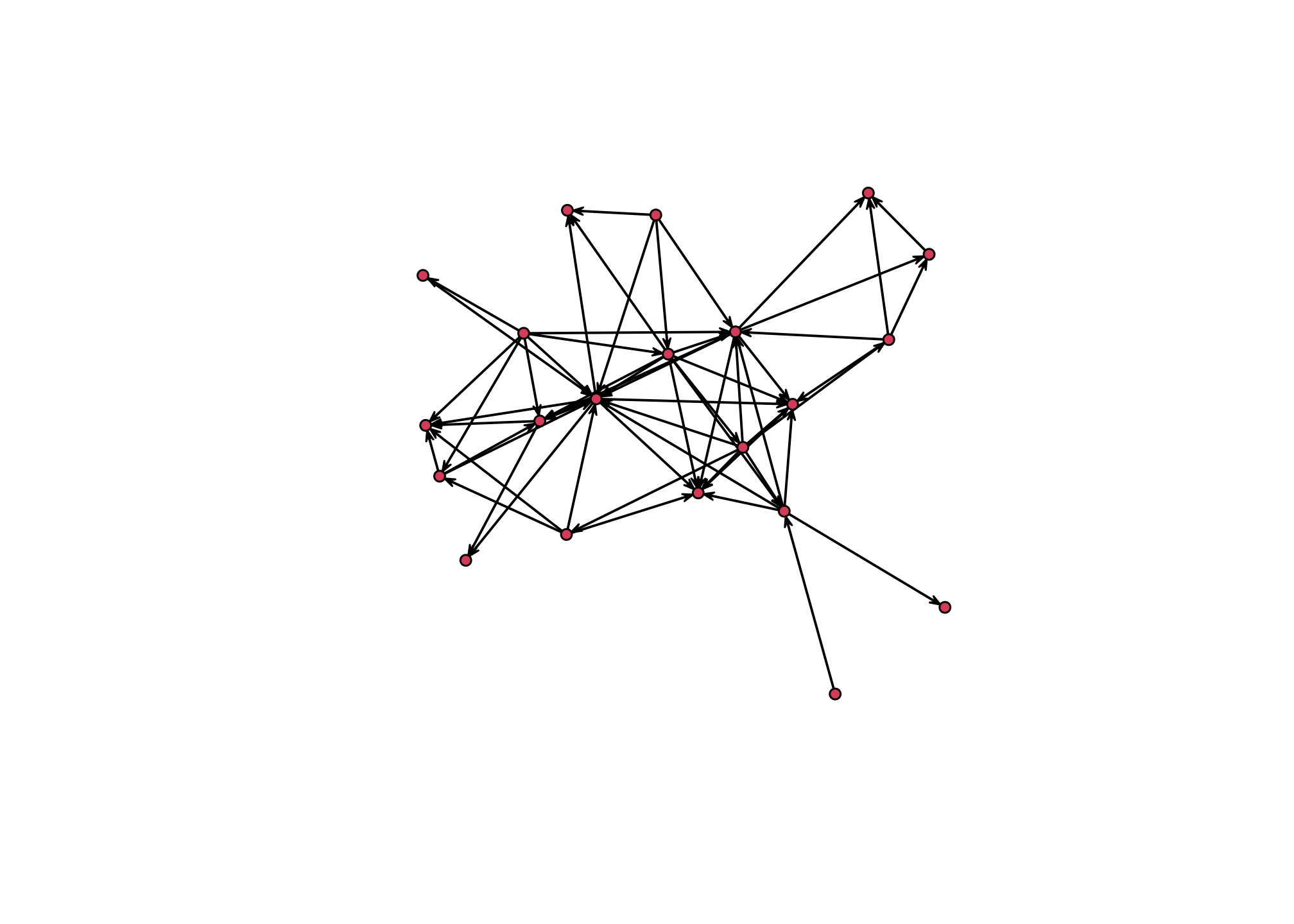
possibly with larger vertices
plot(starwars_network,
     vertex.cex = 3)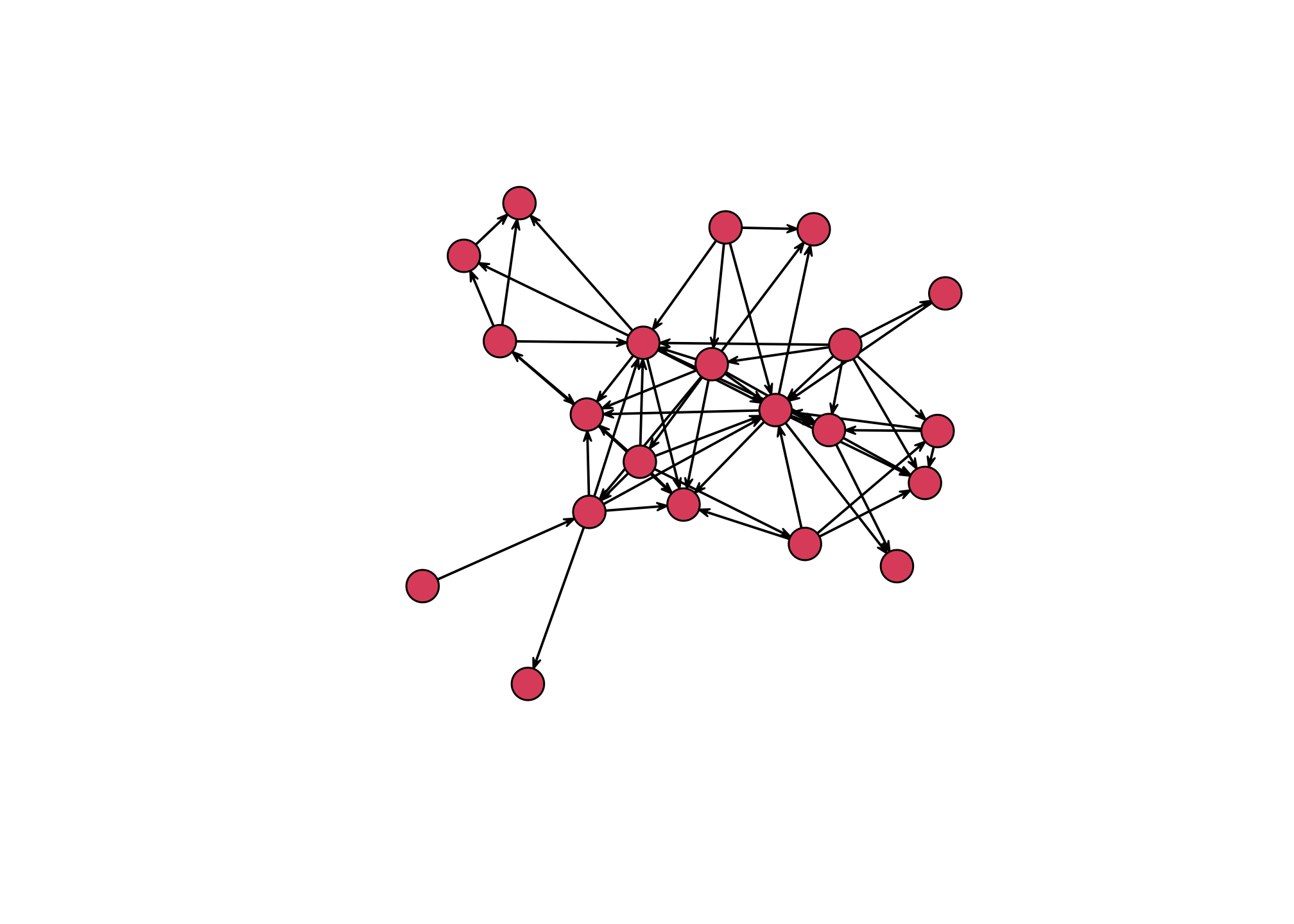
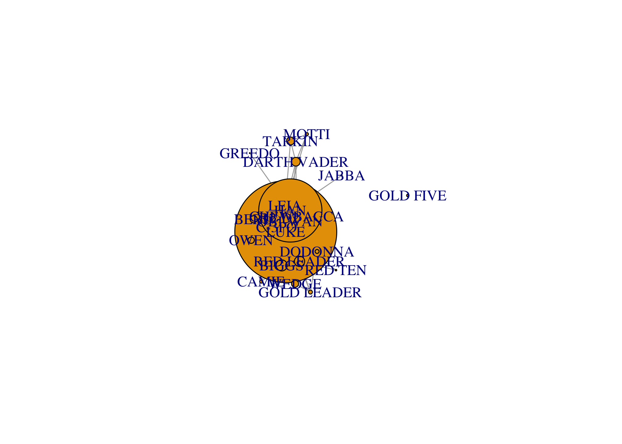
and into a particular structure as well
plot(starwars_network,
     vertex.cex = 3,
     mode = "circle")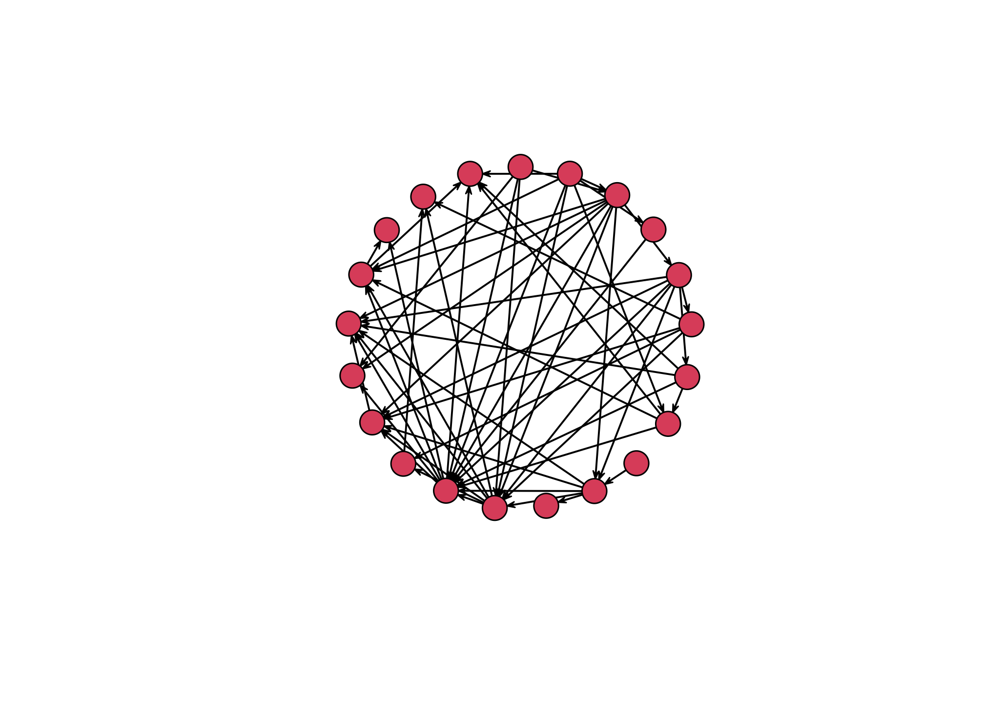
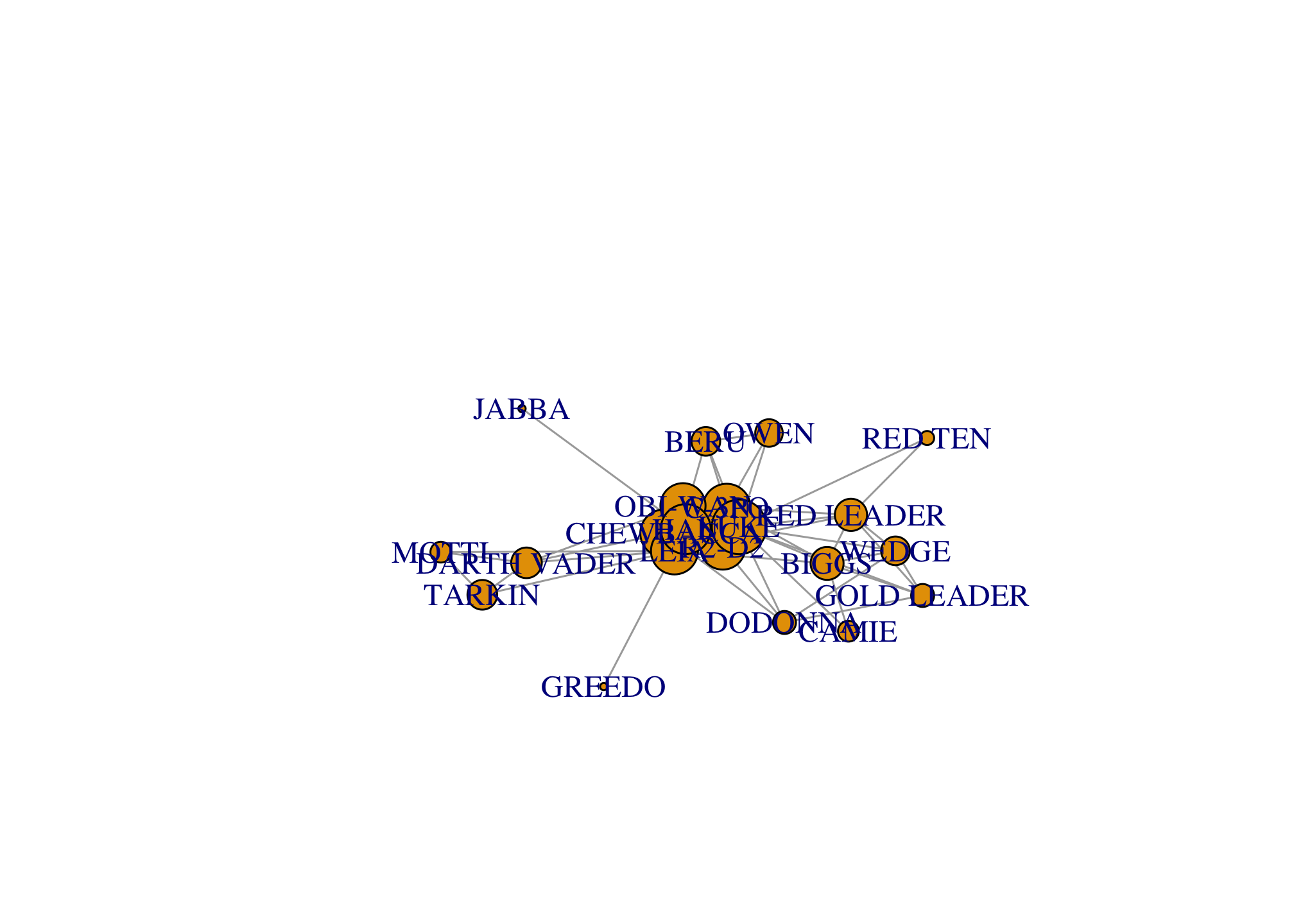
or
plot(starwars_network,
     vertex.cex = 3,
     mode = "kamadakawai")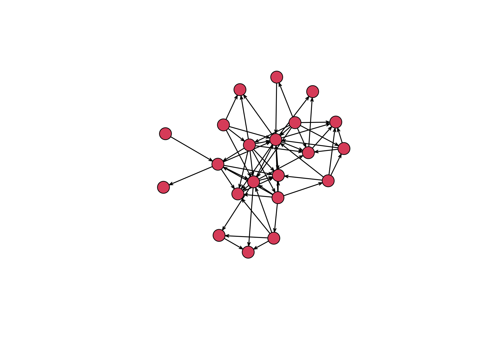
if you prefer.
The tidygraph and ggraph packages
Please install and load the following package
library(tidygraph)##
## Attaching package: 'tidygraph'## The following object is masked from 'package:igraph':
##
## groups## The following object is masked from 'package:stats':
##
## filterlibrary(ggraph)Two important piece of information are that
Nearly all network analysis packages are based on
igraphbut thenetworkpackage is not one of them.The
networkpackage actually causes a lot of conflicts withigraphso we need to unload it and any information based on it by running
detach(package:network)and
rm(starwars_network)The tidiest packages that you can use to perform network analyses are tidygraph and ggraph.
So let’s first create a network object using tidygraph which uses a similar approach as igraph
starwars_tidy <-
  tbl_graph(nodes = nodes,
            edges = edges,
            directed = FALSE)
We can again verify the class by
class(starwars_tidy)## [1] "tbl_graph" "igraph"Let’s take a look at the underlying information
starwars_tidy## # A tbl_graph: 22 nodes and 60 edges
## #
## # An undirected simple graph with 2 components
## #
## # Node Data: 22 x 3 (active)
## name id allegiance
## <chr> <dbl> <chr>
## 1 R2-D2 0 Galactic Republic
## 2 CHEWBACCA 1 Galactic Republic
## 3 C-3PO 2 Galactic Republic
## 4 LUKE 3 Jedi Order
## 5 DARTH VADER 4 Sith Order
## 6 CAMIE 5 Unknown
## # … with 16 more rows
## #
## # Edge Data: 60 x 3
## from to weight
## <int> <int> <dbl>
## 1 1 3 17
## 2 1 4 13
## 3 1 11 6
## # … with 57 more rowsNotice that the package is built on igraph!
Note from the output that the nodes are active. This is what is known as an active tibble within a tbl_graph object and makes it possible to manipulate the data in one tibble at a time. The nodes tibble is activated by default, but you can change which tibble is active with the activate() function. Thus, if I wanted to rearrange the rows in the edges tibble to list those with the highest weight first, I could use activate() and then arrange() like so
starwars_tidy %>%
  activate(edges) %>%
  arrange(desc(weight))
## # A tbl_graph: 22 nodes and 60 edges
## #
## # An undirected simple graph with 2 components
## #
## # Edge Data: 60 x 3 (active)
## from to weight
## <int> <int> <dbl>
## 1 4 14 26
## 2 2 14 19
## 3 4 11 19
## 4 3 4 18
## 5 1 3 17
## 6 4 8 17
## # … with 54 more rows
## #
## # Node Data: 22 x 3
## name id allegiance
## <chr> <dbl> <chr>
## 1 R2-D2 0 Galactic Republic
## 2 CHEWBACCA 1 Galactic Republic
## 3 C-3PO 2 Galactic Republic
## # … with 19 more rowsThe tidy approach is relatively simple so lets plot it
ggraph(starwars_tidy) +
  geom_edge_link() +
  geom_node_point() +
  theme_graph()
## Using `stress` as default layout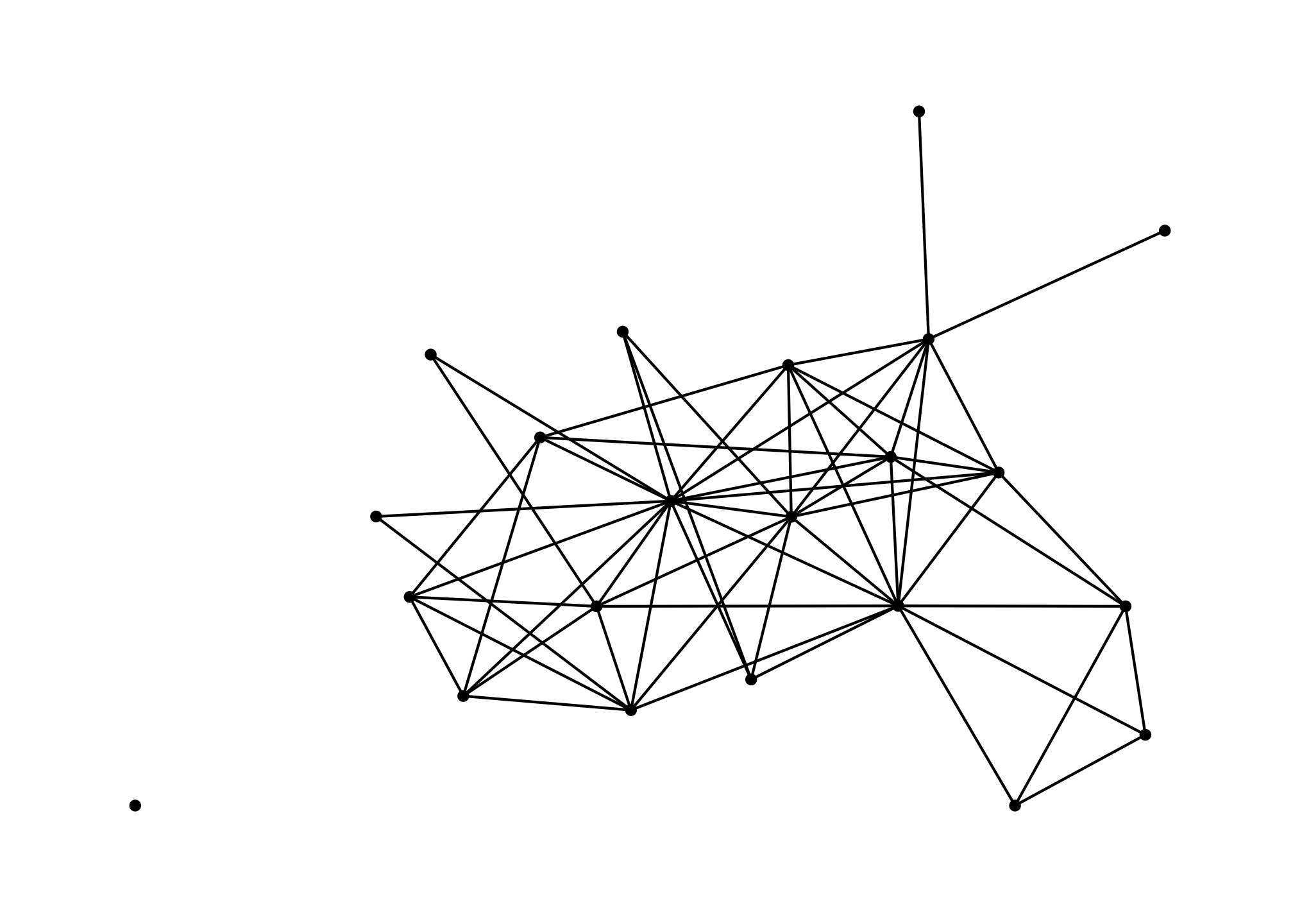
This uses a default layout called stress but there are any others which you can find here. Yes it is also absolutely similar to ggplot which allows us to use all kinds of common packages and functions
ggraph(starwars_tidy,
layout = "graphopt") +
geom_edge_link(aes(width = weight),
alpha = 0.5,
show.legend = FALSE) +
scale_edge_width(range = c(0.2, 1.2)) +
geom_node_point(aes(size = centrality_pagerank(),
fill = centrality_degree()),
shape = 21,
stroke = 1.4,
color = "#4d194d",
show.legend = FALSE) +
scale_size(range = c(1, 14)) +
scale_fill_gradient(low = "#81b29a", high = "#3d405b") +
geom_node_label(aes(label = name),
repel = TRUE) +
coord_fixed() +
theme_graph()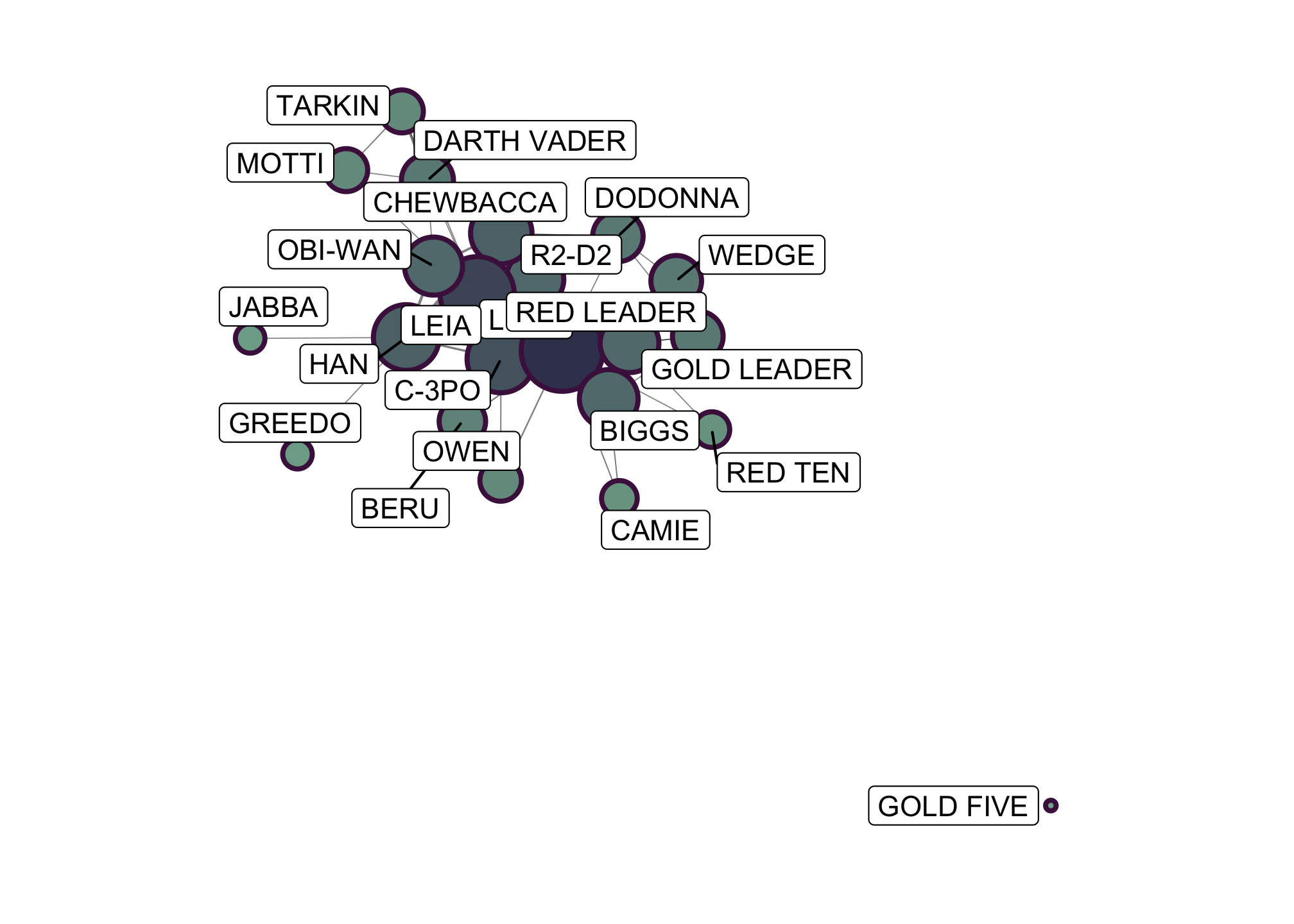 and do fun things with the data
ggraph(starwars_tidy,
       layout = "linear",
       circular = TRUE) +
  geom_edge_arc(aes(width = weight,
                    color = weight),
                alpha = 0.8,
                show.legend = FALSE) +
  scale_edge_width(range = c(0.2, 2)) +
  scale_edge_color_gradient(low = "#b7094c", high = "#0091ad") +
  geom_node_label(aes(label = name,
                      size = centrality_betweenness()),
                  show.legend = FALSE) +
  scale_size(range = c(3, 6)) +
  theme_graph()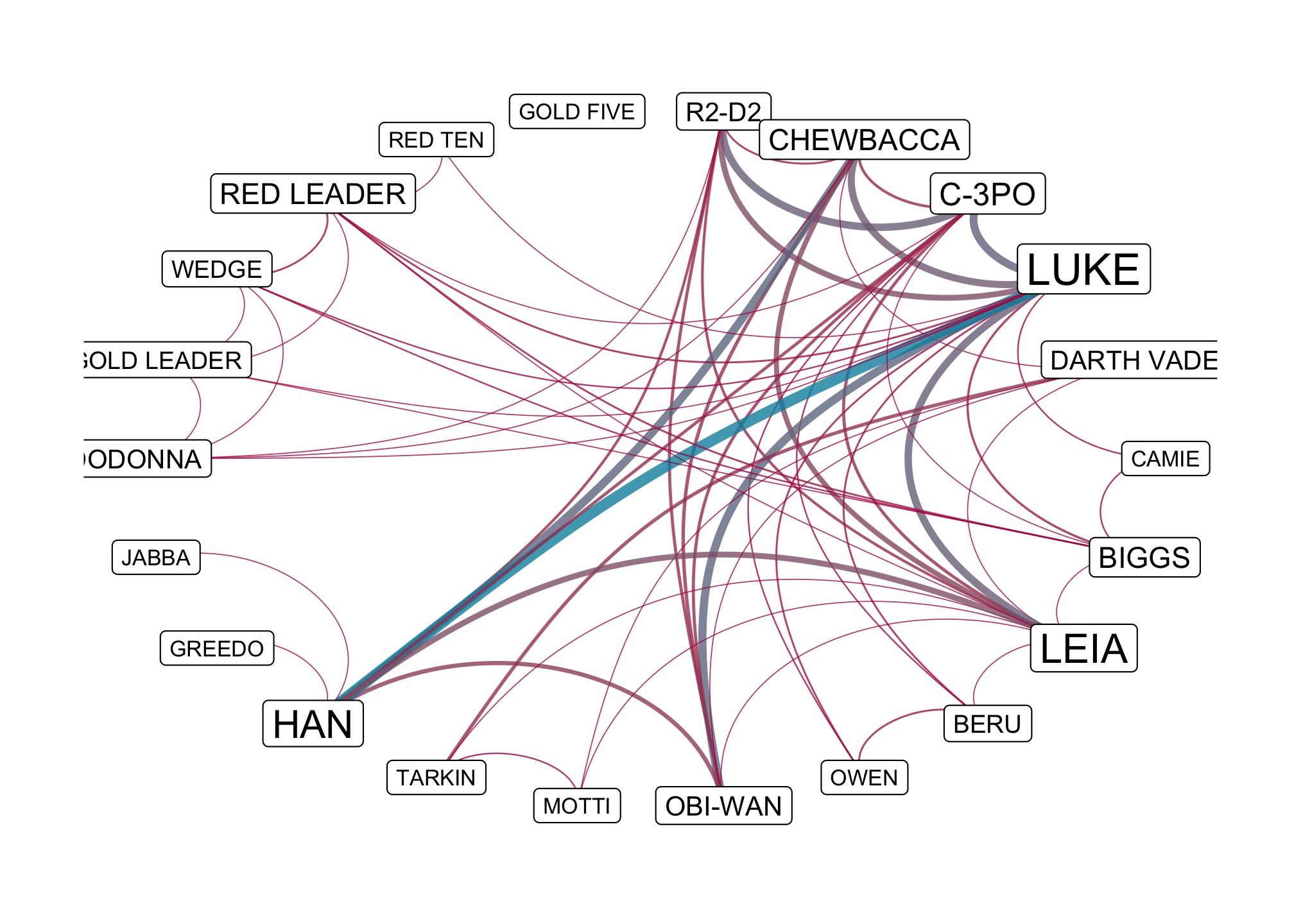
Interactive network graphs with visNetwork and networkD3
Please install and load the following package
library(visNetwork)
library(networkD3)
visNetwork
The visNetwork() package uses a nodes list and edges list to create an interactive graph and it is picky! Here are the requirements
- from the
nodedata set- must include an id column
- names of the nodes must come from the label column5
- from the
edgedata set- must have from and to columns.
The network is fun to play around with. With just the basic plot, you can
- move the nodes and the graph will use an algorithm to keep the nodes properly spaced.
- zoom in and out on the plot and move it around to re-center it
So we can grab the edge set
edge_list <-
  starwars_tidy %>%
    activate(edges) %>%
    data.frame()
Take a look
edge_list## from to weight
## 1 1 3 17
## 2 1 4 13
## 3 1 11 6
## 4 1 8 5
## 5 1 14 5
## 6 1 2 3
## 7 1 17 1
## 8 2 11 7
## 9 2 3 5
## 10 2 4 16
## 11 2 14 19
## 12 2 8 11
## 13 2 5 1
## 14 2 17 1
## 15 4 6 2
## 16 6 7 2
## 17 4 7 4
## 18 5 8 1
## 19 4 9 3
## 20 9 10 3
## 21 3 9 2
## 22 4 10 3
## 23 3 4 18
## 24 3 10 2
## 25 3 8 6
## 26 4 8 17
## 27 8 9 1
## 28 4 11 19
## 29 3 11 6
## 30 8 11 1
## 31 12 13 2
## 32 5 12 1
## 33 5 13 7
## 34 11 14 9
## 35 4 14 26
## 36 14 15 1
## 37 14 16 1
## 38 3 14 6
## 39 8 12 1
## 40 8 13 1
## 41 8 14 13
## 42 5 11 1
## 43 17 18 1
## 44 17 19 1
## 45 4 17 1
## 46 18 19 1
## 47 4 18 1
## 48 4 19 2
## 49 7 8 1
## 50 8 20 1
## 51 4 20 3
## 52 7 20 3
## 53 3 7 1
## 54 3 20 1
## 55 19 20 3
## 56 18 20 1
## 57 7 19 2
## 58 20 21 1
## 59 7 18 1
## 60 4 21 1And manipulate the node a bit
node_list <-
  starwars_tidy %>%
    activate(nodes) %>%
    data.frame() %>%
    rename(label = name) %>%
    rename(group = allegiance)
Take a look
node_list## label id group
## 1 R2-D2 0 Galactic Republic
## 2 CHEWBACCA 1 Galactic Republic
## 3 C-3PO 2 Galactic Republic
## 4 LUKE 3 Jedi Order
## 5 DARTH VADER 4 Sith Order
## 6 CAMIE 5 Unknown
## 7 BIGGS 6 Galactic Republic
## 8 LEIA 7 Galactic Republic
## 9 BERU 8 Galactic Republic
## 10 OWEN 9 Galactic Republic
## 11 OBI-WAN 10 Jedi Order
## 12 MOTTI 11 Galactic Empire
## 13 TARKIN 12 Galactic Empire
## 14 HAN 13 Galactic Republic
## 15 GREEDO 14 Hutt Cartel
## 16 JABBA 15 Hutt Cartel
## 17 DODONNA 16 Galactic Republic
## 18 GOLD LEADER 17 Galactic Republic
## 19 WEDGE 18 Galactic Republic
## 20 RED LEADER 19 Galactic Republic
## 21 RED TEN 20 Galactic Republic
## 22 GOLD FIVE 21 Galactic Republicand plot it
visNetwork(node_list,
           edge_list)
Let’s work on the aesthetics of the nodes
new_node_list <- node_list %>%
                  mutate(borderWidth = 1.5) %>%
                  mutate(color.background =
                           case_when(
                             group == "Galactic Republic" ~ "#CF6728",
                             group == "Jedi Order" ~ "#4BA1F0",
                             group == "Galactic Empire" ~ "#741D2F",
                             group == "Sith Order" ~ "#912721",
                             group == "Hutt Cartel" ~ "#c3cb71",
                             group == "Unknown" ~ "#5a5255"
                           )
                  ) %>%
                  mutate(color.border = "#43675a") %>%
                  mutate(color.highlight.border = "#3a95a7") %>%
                  mutate(font.color = "#FFFFFF")
and weight the edges for no good reason
weighted_edges <- mutate(edge_list,
                         width = weight/4 + 1)
weighted_edges ## from to weight width
## 1 1 3 17 5.25
## 2 1 4 13 4.25
## 3 1 11 6 2.50
## 4 1 8 5 2.25
## 5 1 14 5 2.25
## 6 1 2 3 1.75
## 7 1 17 1 1.25
## 8 2 11 7 2.75
## 9 2 3 5 2.25
## 10 2 4 16 5.00
## 11 2 14 19 5.75
## 12 2 8 11 3.75
## 13 2 5 1 1.25
## 14 2 17 1 1.25
## 15 4 6 2 1.50
## 16 6 7 2 1.50
## 17 4 7 4 2.00
## 18 5 8 1 1.25
## 19 4 9 3 1.75
## 20 9 10 3 1.75
## 21 3 9 2 1.50
## 22 4 10 3 1.75
## 23 3 4 18 5.50
## 24 3 10 2 1.50
## 25 3 8 6 2.50
## 26 4 8 17 5.25
## 27 8 9 1 1.25
## 28 4 11 19 5.75
## 29 3 11 6 2.50
## 30 8 11 1 1.25
## 31 12 13 2 1.50
## 32 5 12 1 1.25
## 33 5 13 7 2.75
## 34 11 14 9 3.25
## 35 4 14 26 7.50
## 36 14 15 1 1.25
## 37 14 16 1 1.25
## 38 3 14 6 2.50
## 39 8 12 1 1.25
## 40 8 13 1 1.25
## 41 8 14 13 4.25
## 42 5 11 1 1.25
## 43 17 18 1 1.25
## 44 17 19 1 1.25
## 45 4 17 1 1.25
## 46 18 19 1 1.25
## 47 4 18 1 1.25
## 48 4 19 2 1.50
## 49 7 8 1 1.25
## 50 8 20 1 1.25
## 51 4 20 3 1.75
## 52 7 20 3 1.75
## 53 3 7 1 1.25
## 54 3 20 1 1.25
## 55 19 20 3 1.75
## 56 18 20 1 1.25
## 57 7 19 2 1.50
## 58 20 21 1 1.25
## 59 7 18 1 1.25
## 60 4 21 1 1.25and plot it
visNetwork(new_node_list,
           weighted_edges,
           height = "700px",
           width = "100%") %>%
  visEdges(color = "#c7bbc9") %>%
  visNodes(shape = "circle",
           color = list(hover = "#5cb85c",
                        highlight = "#449d44"),
           shadow = list(enabled = TRUE,
                         size = 5))  %>%
  visInteraction(navigationButtons = TRUE,
                 hover = TRUE) %>%
  visOptions(selectedBy = "group",
             highlightNearest = TRUE,
             nodesIdSelection = TRUE,
             collapse = TRUE) %>%
  visPhysics(solver = "repulsion",
             repulsion = list(nodeDistance = 400,
                              springlength = 300,
                              centralGravity = 0.2),
             timestep = 0.75,
             stabilization = TRUE) %>%
  visPhysics(stabilization = FALSE)   %>%
  visLayout(randomSeed = 12)
We can even group them
node_list_byside <-
        starwars_tidy %>%
          activate(nodes) %>%
          data.frame() %>%
          rename(label = name)
networkD3
A little wrangling is necessary to prepare the data to create a networkD3 graph. To make a networkD3 graph with a edge and node list requires that the IDs be a series of numeric integers that begin with 0.
nodes_d3 <- mutate(node_list,
                   id = id - 1)

edges_d3 <- mutate(edge_list,
                   from = from - 1,
                   to = to - 1)
and we can plot it
forceNetwork(Links = edges_d3,
             Nodes = nodes_d3,
             Source = "from",
             Target = "to",
             NodeID = "label",
             Group = "id",
             Value = "weight",
             opacity = 1,
             fontSize = 16,
             zoom = TRUE)
or you can see how the individual nodes are linked
sankeyNetwork(Links = edges_d3,
              Nodes = nodes_d3,
              Source = "from",
              Target = "to",
              NodeID = "label",
              Value = "weight",
              fontSize = 16,
              unit = "Letter(s)")
Consider just pasting it at the top of your script and leaving it there. Please note that this will not work in an Rmarkdown file or Shiny app.↩︎
Typically indicates importance.↩︎
Note that everything in this data set is weighted so the weight is not shown. However we could add another column with just weights if there was a reason to do so like force users get a weight of
2abd everyone else receives a1.↩︎We’ll expand on this in a bit.↩︎
If you intend to use labels.↩︎
