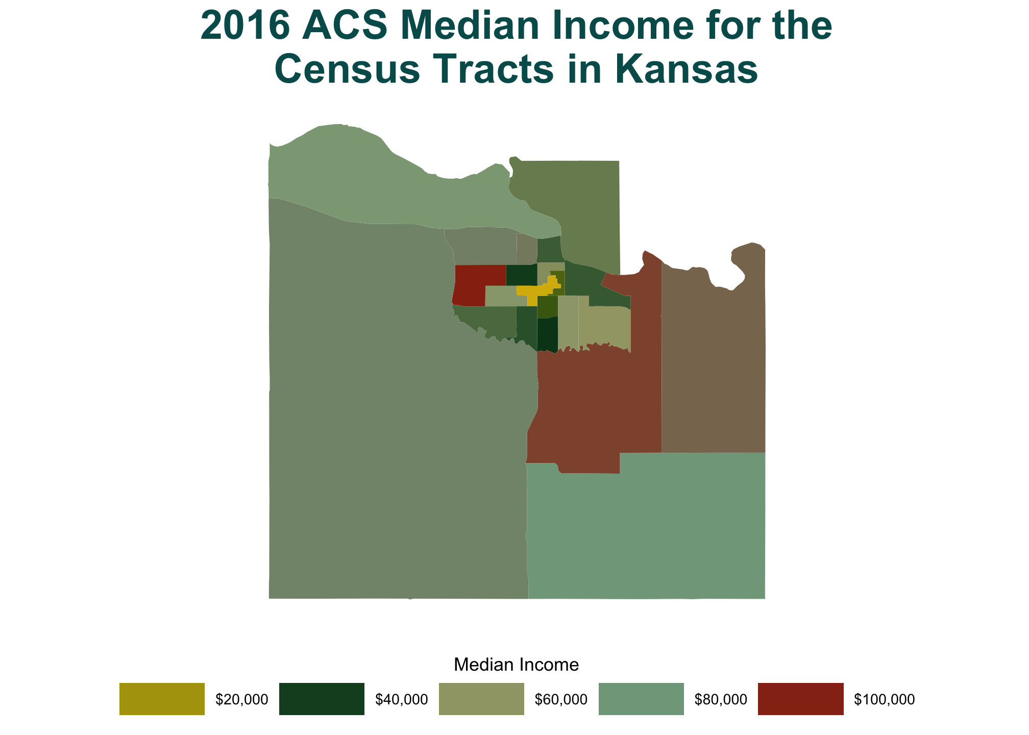
I'm the Map
Getting Prepped
Possible Solutions
Remember just because your code doesn’t look like mine doesn’t mean anything. Included are examples of approaches that can be used to complete this task, but there are so many more!
library(tidyverse)
library(tidycensus)
library(DT)
library(wesanderson)
library(ggthemes)
library(scales)First let’s check the FIPS codes for the states and counties
head(tidycensus::fips_codes)## state state_code state_name county_code county
## 1 AL 01 Alabama 001 Autauga County
## 2 AL 01 Alabama 003 Baldwin County
## 3 AL 01 Alabama 005 Barbour County
## 4 AL 01 Alabama 007 Bibb County
## 5 AL 01 Alabama 009 Blount County
## 6 AL 01 Alabama 011 Bullock CountyPrior Things
Data Set
For the following, we’ll use a single variable though you can absolutely use many more! In this case, let’s utilize the average income measured by medians in 2016.
vars_of_interest <- c(median_income = "B19013_001")Color Palettes
We will need continuous color palettes to display the data well. In this case we’ll use the wesanderson collection, but please feel free to use your own.
National Level Data
national_data <- get_acs(geography = "county",
variables = vars_of_interest,
year = 2016,
survey = "acs5",
shift_geo = TRUE,
geometry = TRUE) %>%
rename(`Median Income` = estimate)Make sure to check it
datatable(national_data) Let’s now create a palette
wes_palette("Darjeeling2")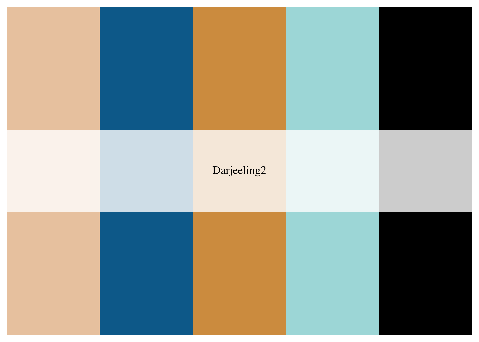
make it continuous
darj2 <- wes_palette("Darjeeling2",
max(national_data$`Median Income`,
na.rm = TRUE),
type = "continuous")and plot it for the entire US
ggplot() +
geom_sf(data = national_data,
mapping = aes(fill = `Median Income`),
color = NA) +
coord_sf(datum = NA) +
scale_fill_gradientn(colors = darj2) +
theme_minimal() +
theme(plot.title = element_text(size = 20,
face = "bold",
color = "#005b5b",
hjust = 0.5)) +
ggtitle(stringr::str_wrap("2016 ACS Median Income for the United States", 35))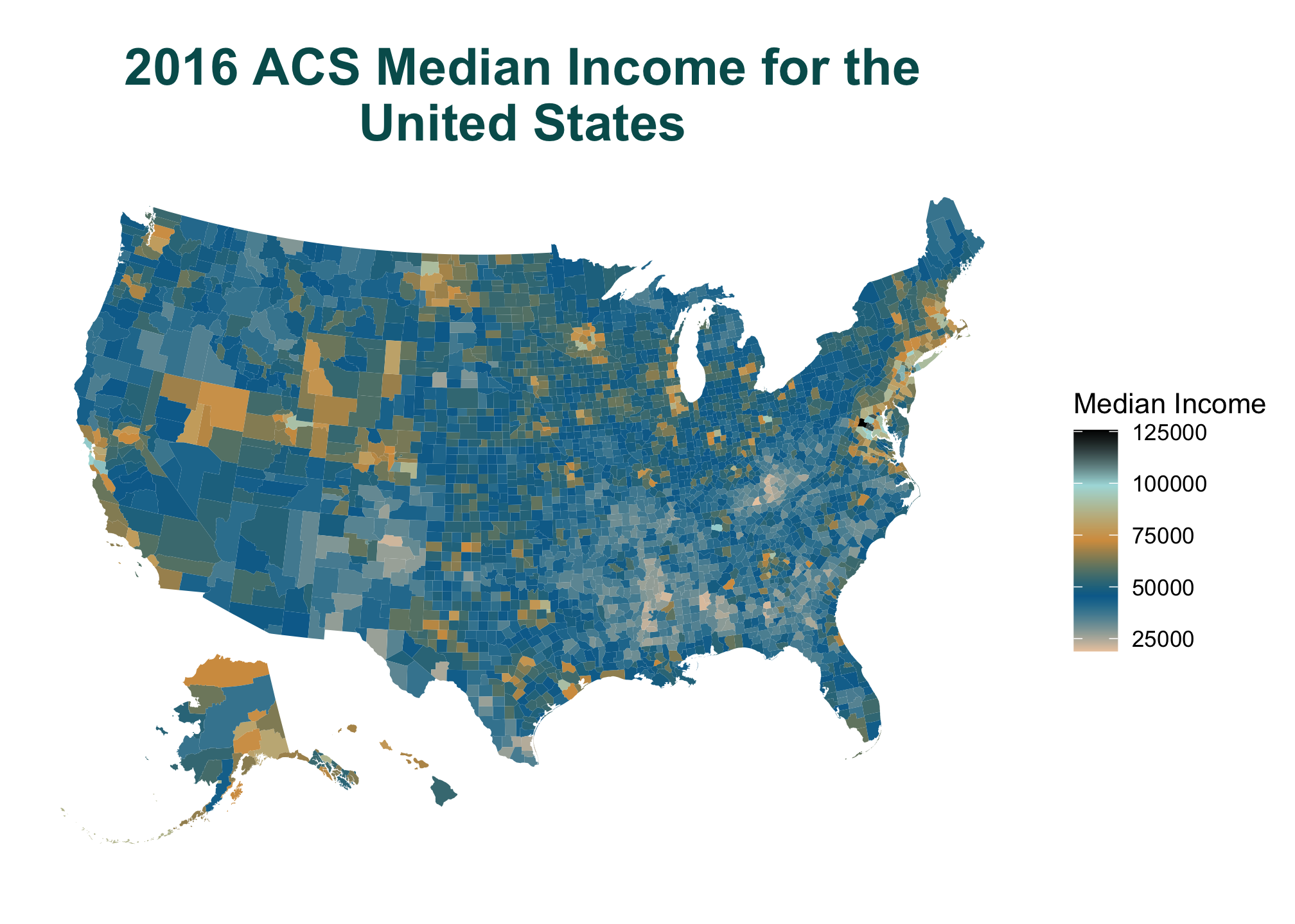
Regional Level Data
Here is a US Census PDF of what the regions are. Now Region 1 can be defined by
region1 = c("CT", "ME", "MA", "NH", "RI", "VT", "NJ", "NY", "PA")We get acs data and geographies for our variable at the
- tract level
multistate_tract_data <- get_acs(geography = "tract",
variables = vars_of_interest,
state = region1,
year = 2016,
survey = "acs5",
geometry = TRUE) %>%
rename(`Median Income` = estimate)Make sure to check it
datatable(multistate_tract_data) | GEOID | NAME | variable | Median Income | moe | geometry |
|---|---|---|---|---|---|
| 09001011000 | Census Tract 110, Fairfield County, Connecticut | median_income | 248171 | 33760 | MULTIPOLYGON (((-73.58765 4… |
| 09001020800 | Census Tract 208, Fairfield County, Connecticut | median_income | 134934 | 15960 | MULTIPOLYGON (((-73.54896 4… |
| 09001021400 | Census Tract 214, Fairfield County, Connecticut | median_income | 55101 | 7886 | MULTIPOLYGON (((-73.56834 4… |
| 09001022200 | Census Tract 222, Fairfield County, Connecticut | median_income | 58889 | 10637 | MULTIPOLYGON (((-73.54503 4… |
| 09001043100 | Census Tract 431, Fairfield County, Connecticut | median_income | 125536 | 31382 | MULTIPOLYGON (((-73.47108 4… |
| 09001045400 | Census Tract 454, Fairfield County, Connecticut | median_income | 189375 | 38749 | MULTIPOLYGON (((-73.42248 4… |
- state level
multistate_state_data <- get_acs(geography = "state",
variables = vars_of_interest,
state = region1,
year = 2016,
survey = "acs5",
geometry = TRUE) %>%
rename(`Median Income` = estimate)Make sure to check it
datatable(multistate_state_data) | GEOID | NAME | variable | Median Income | moe | geometry |
|---|---|---|---|---|---|
| 09001011000 | Census Tract 110, Fairfield County, Connecticut | median_income | 248171 | 33760 | MULTIPOLYGON (((-73.58765 4… |
| 09001020800 | Census Tract 208, Fairfield County, Connecticut | median_income | 134934 | 15960 | MULTIPOLYGON (((-73.54896 4… |
| 09001021400 | Census Tract 214, Fairfield County, Connecticut | median_income | 55101 | 7886 | MULTIPOLYGON (((-73.56834 4… |
| 09001022200 | Census Tract 222, Fairfield County, Connecticut | median_income | 58889 | 10637 | MULTIPOLYGON (((-73.54503 4… |
| 09001043100 | Census Tract 431, Fairfield County, Connecticut | median_income | 125536 | 31382 | MULTIPOLYGON (((-73.47108 4… |
| 09001045400 | Census Tract 454, Fairfield County, Connecticut | median_income | 189375 | 38749 | MULTIPOLYGON (((-73.42248 4… |
Putting geometry = TRUE brings in the geographic information (aka shapefiles) so make sure that is on, though if you only need the data and not a map, save yourself some time and turn it off. Geographic data is relatively dense and can take some time depending on how much you need.
Optionally let’s create a palette,
wes_palette("Darjeeling1")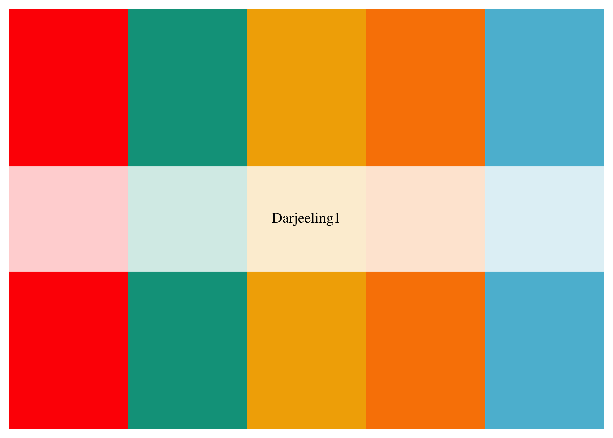
make it continuous
darj1 <- wes_palette("Darjeeling1",
max(multistate_tract_data$`Median Income`,
na.rm = TRUE),
type = "continuous")and plot it. This is tract level data so you’ll have to wait a little bit
ggplot() +
geom_sf(data = multistate_tract_data,
mapping = aes(fill = `Median Income`),
color = NA) +
scale_fill_gradientn(colors = darj1) +
theme_map() 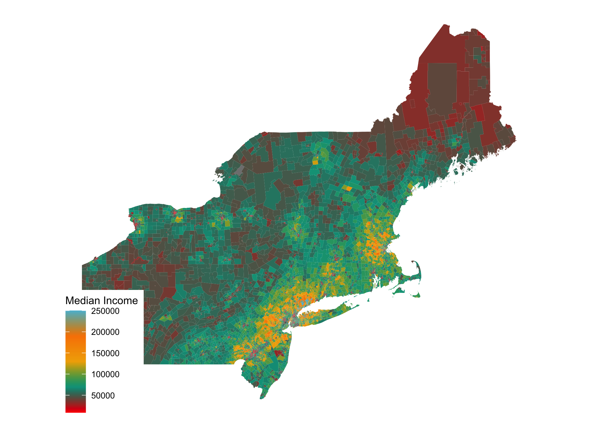
Let’s give it a go with state borders so its a bit more familiar and with a formatted title and some finagling of the legend
ggplot() +
geom_sf(data = multistate_tract_data,
mapping = aes(fill = `Median Income`),
color = NA) +
geom_sf(data = multistate_state_data,
color = "#f7f7f7",
fill = NA) +
scale_fill_gradientn(colors = darj1,
label = scales::dollar) +
theme_map() +
theme(plot.title = element_text(size = 20,
face = "bold",
color = "#005b5b",
hjust = 0.5),
legend.position = c(0.8,0.1),
legend.title = element_text(size = 12,
face = "bold",
color = "#3392a4",
hjust = 0.5,
margin = margin(b = 10)),
legend.text = element_text(size = 10,
face = "bold",
color = "#2d8292")) +
ggtitle("2016 ACS Median Income for Census Region 1")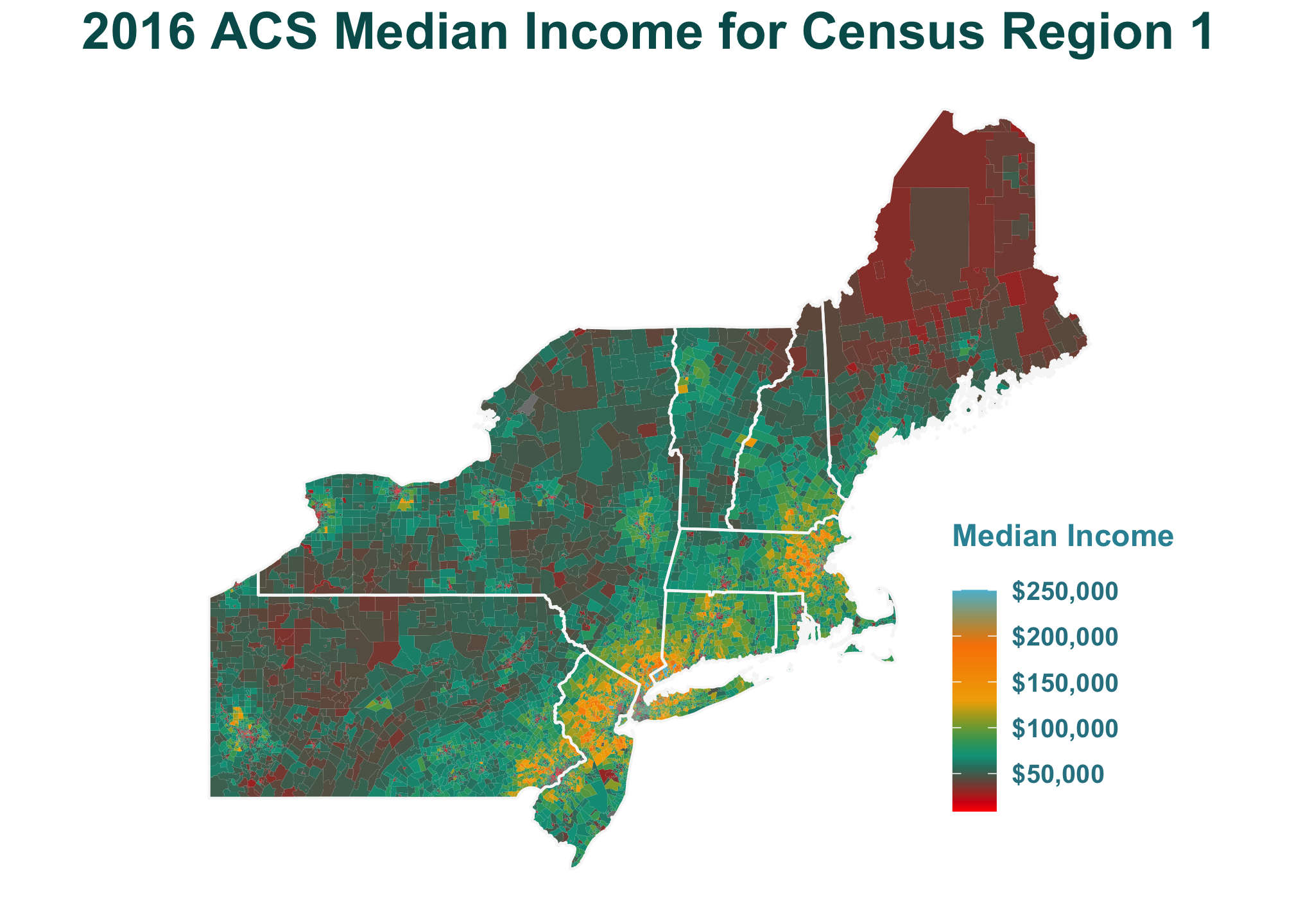
State Level Data
We get acs data and geographies for our variable using
state_data <- get_acs(geography = "state",
variables = vars_of_interest,
year = 2016,
survey = "acs5",
shift_geo = TRUE,
geometry = TRUE) %>%
rename(`Median Income` = estimate)Make sure to check it
datatable(state_data) Optionally let’s create a palette,
wes_palette("Zissou1")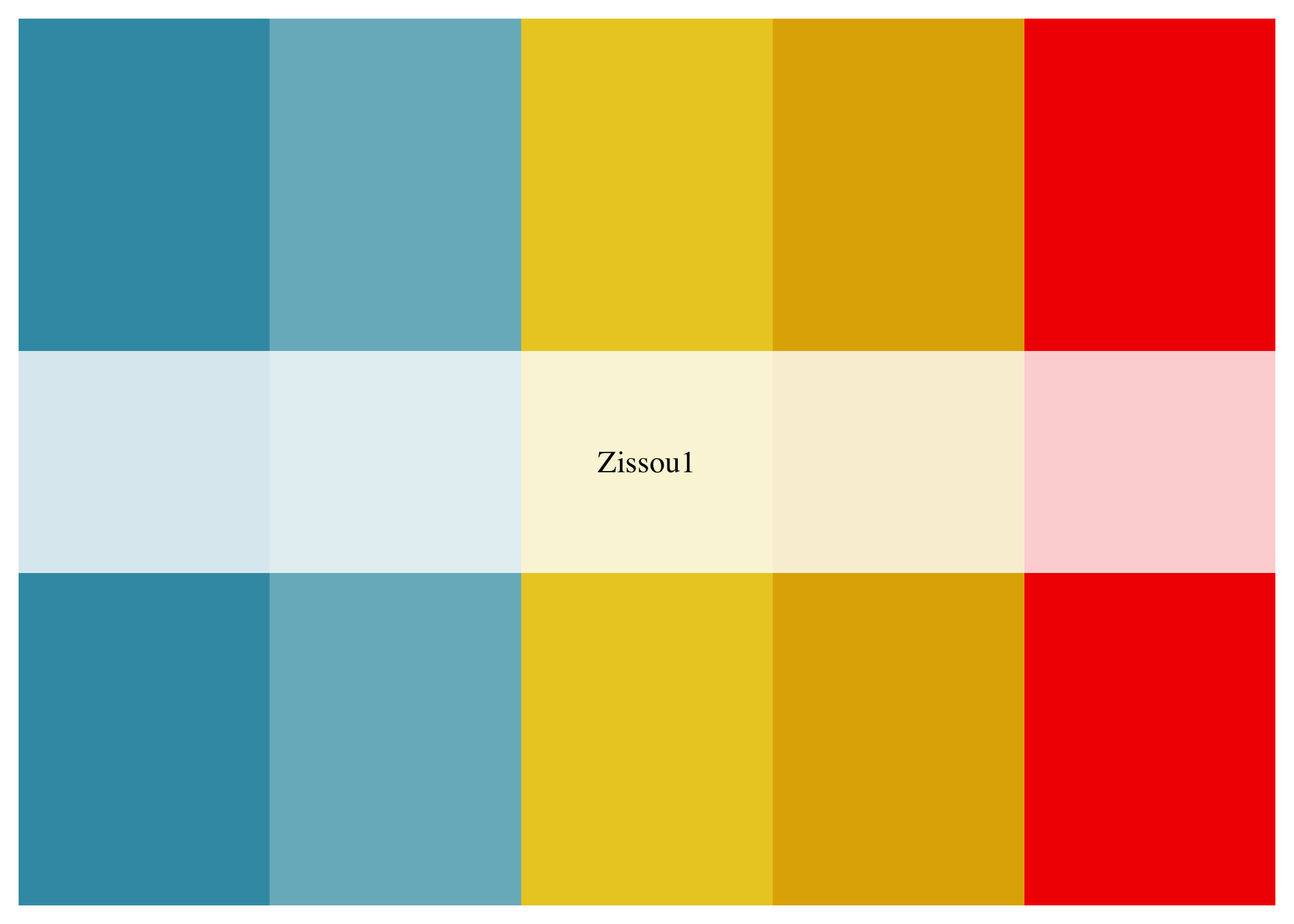
make it continuous
ziss1 <- wes_palette("Zissou1",
max(state_data$`Median Income`,
na.rm = TRUE),
type = "continuous")and plot it for the entire US
ggplot() +
geom_sf(data = state_data,
mapping = aes(fill = `Median Income`),
color = NA) +
scale_fill_gradientn(colors = ziss1) +
theme_map() +
theme(plot.title = element_text(size = 20,
face = "bold",
color = "#005b5b",
hjust = 0.5)) +
ggtitle("2016 ACS Median Income for All US States")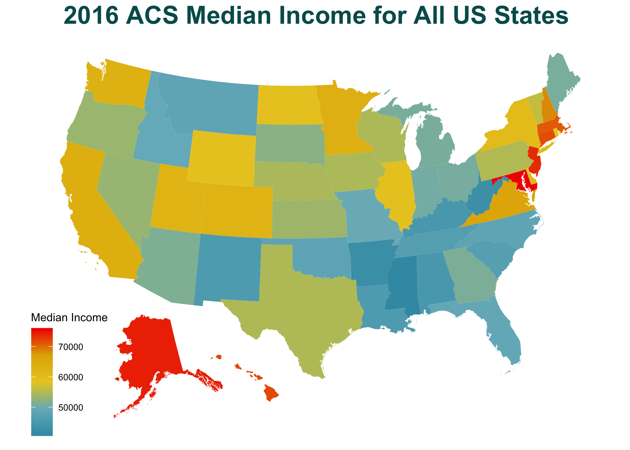
or just the lower 48 states
lower_48 <- state_data %>%
filter(GEOID < 60) %>%
filter(!NAME == "Hawaii") %>%
filter(!NAME == "Alaska")ggplot() +
geom_sf(data = lower_48,
mapping = aes(fill = `Median Income`),
color = NA) +
scale_fill_gradientn(colors = ziss1) +
theme_map() +
coord_sf(crs = 5070,
datum = NA) +
theme(plot.title = element_text(size = 20,
face = "bold",
color = "#005b5b",
hjust = 0.5)) +
ggtitle(stringr::str_wrap("2016 ACS Median Income for the Contiguous US States", 35))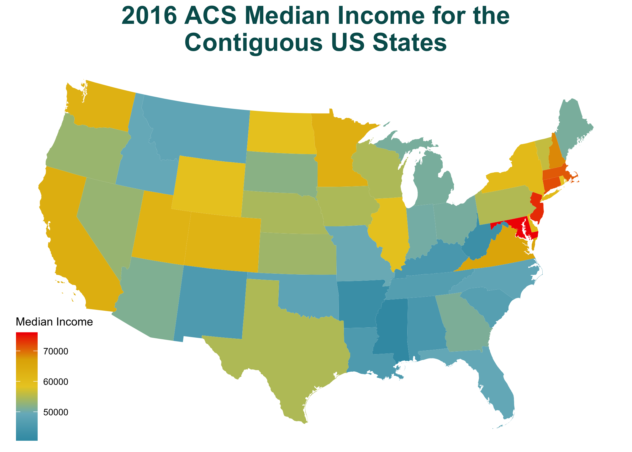
County Level Data
Tract level data is sometimes tricky to get, in that not all data sets with geographies have them. Sticking to the widespread surveys such as the decennial census and acs will always work, while others are up in the air.
kansas <- get_acs(state = "KS",
geography = "county",
variables = vars_of_interest,
geometry = TRUE) %>%
rename(`Median Income` = estimate)datatable(kansas)| GEOID | NAME | variable | Median Income | moe | geometry |
|---|---|---|---|---|---|
| 20099 | Labette County, Kansas | median_income | 47643 | 2802 | MULTIPOLYGON (((-95.52265 3… |
| 20203 | Wichita County, Kansas | median_income | 57978 | 7215 | MULTIPOLYGON (((-101.5671 3… |
| 20077 | Harper County, Kansas | median_income | 49865 | 2945 | MULTIPOLYGON (((-98.3498 37… |
| 20093 | Kearny County, Kansas | median_income | 52599 | 10953 | MULTIPOLYGON (((-101.5419 3… |
| 20069 | Gray County, Kansas | median_income | 64930 | 3363 | MULTIPOLYGON (((-100.665 37… |
| 20161 | Riley County, Kansas | median_income | 51208 | 2475 | MULTIPOLYGON (((-96.96095 3… |
wes_palette("FantasticFox1")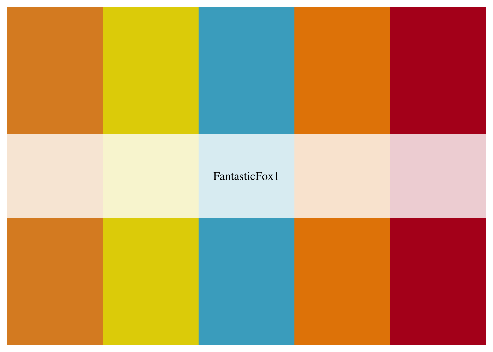
make it continuous
ffox <- wes_palette("FantasticFox1",
max(kansas$`Median Income`,
na.rm = TRUE),
type = "continuous")and plot it!
kansas %>%
ggplot(aes(fill = `Median Income`)) +
geom_sf(color = NA) +
scale_fill_gradientn(colors = ffox,
label = scales::dollar) +
theme_map() +
theme(legend.position = "bottom",
legend.direction = "horizontal",
legend.title.align=0.5) +
guides(fill = guide_legend(title.position="top")) +
theme(plot.title = element_text(size = 20,
face = "bold",
color = "#005b5b",
hjust = 0.5)) +
ggtitle("2016 ACS Median Income for the Counties in Kansas")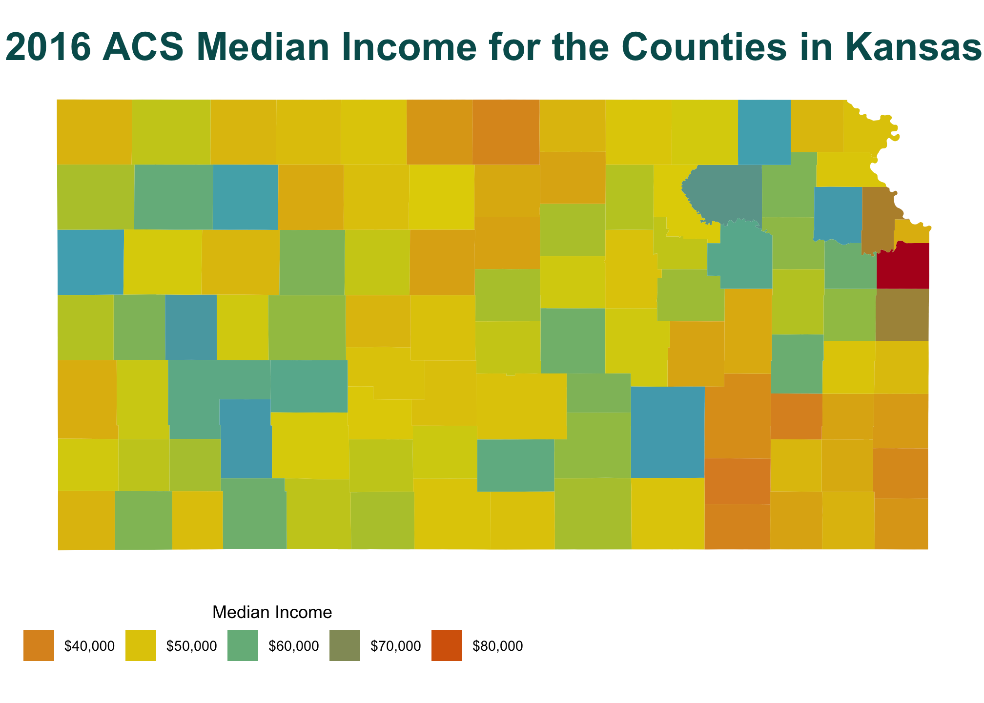
Tract Level Data
Tract level data is sometimes tricky to get, in that not all data sets with geographies have them. Sticking to the widespread surveys such as the decennial census and acs will always work, while others are up in the air.
doug <- get_acs(state = "KS",
county = "Douglas",
geography = "tract",
variables = vars_of_interest,
geometry = TRUE) %>%
rename(`Median Income` = estimate)datatable(doug)| GEOID | NAME | variable | Median Income | moe | geometry |
|---|---|---|---|---|---|
| 20045000901 | Census Tract 9.01, Douglas County, Kansas | median_income | 30353 | 5043 | POLYGON ((-95.26054 38.9359… |
| 20045000502 | Census Tract 5.02, Douglas County, Kansas | median_income | 57035 | 11590 | POLYGON ((-95.2607 38.97286… |
| 20045000501 | Census Tract 5.01, Douglas County, Kansas | median_income | 46952 | 4297 | POLYGON ((-95.261 38.97609,… |
| 20045000604 | Census Tract 6.04, Douglas County, Kansas | median_income | 84536 | 15693 | POLYGON ((-95.2792 38.97794… |
| 20045000300 | Census Tract 3, Douglas County, Kansas | median_income | 28024 | 4766 | POLYGON ((-95.25113 38.9513… |
| 20045000797 | Census Tract 7.97, Douglas County, Kansas | median_income | 64496 | 12992 | POLYGON ((-95.30693 38.957,… |
wes_palette("Cavalcanti1")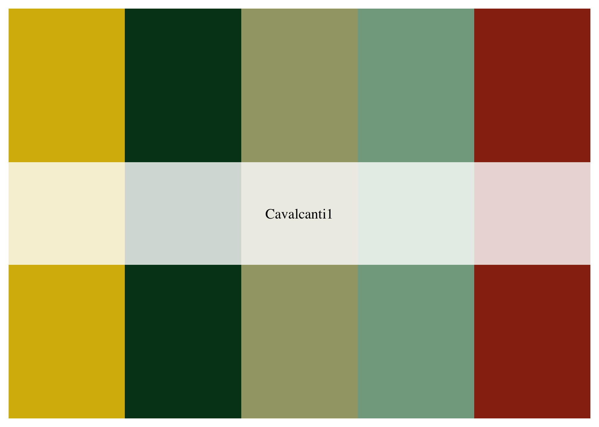
make it continuous
caval <- wes_palette("Cavalcanti1",
max(doug$`Median Income`,
na.rm = TRUE),
type = "continuous")and plot it!
doug %>%
ggplot(aes(fill = `Median Income`)) +
geom_sf(color = NA) +
scale_fill_gradientn(colors = caval,
label = scales::dollar) +
theme_map() +
theme(legend.position = "bottom",
legend.key.width = unit(3, "line")) +
guides(fill = guide_legend(title.position="top",
title.hjust =0.5)) +
theme(plot.title = element_text(size = 20,
face = "bold",
color = "#005b5b",
hjust = 0.5)) +
ggtitle(stringr::str_wrap("2016 ACS Median Income for the Census Tracts in Kansas", 35))